Proving completeness of an eventually perfect failure detector in Lean4

Author: Igor Konnov

Tags: specification lean distributed proofs tlaplus

In the previous blog post, we looked at proving consistency of Two-phase commit in Lean 4. This proof followed the well-trodden path: We found an inductive invariant, quickly model-checked it with Apalache and proved its inductiveness in Lean. One of the immediate questions that I got on X/Twitter was: What about liveness?

Well, liveness of the two-phase commit after the TLA⁺ specification does not seem to be particularly interesting, as it mostly depends on fairness of the resource managers and the transaction manager. (A real implementation may be much trickier though.) I was looking for something a bit more challenging but, at the same time, something that would not take months to reason about. Since many Byzantine-fault tolerance algorithms work under partial synchrony, a natural thing to do was to find a protocol that required partial synchrony. Failure detectors seemed to be a good fit to me. These algorithms are relatively small, but require plenty of reasoning about time.

Hence, I opened the book DP2011 on Reliable and Secure Distributed Programming by Christian Cachin, Rachid Guerraoui, and Luís Rodrigues and found the pseudo-code of the eventually-perfect failure detector (EPFD). If you have never heard of failure detectors, there are a few introductory lectures on YouTube, e.g., this one. Writing a decent TLA⁺-like specification of EPFD and its temporal properties in Lean took me about eight hours. Since temporal properties require us to reason about infinite executions, this required a bit of experimentation with Lean. Figuring out how to capture partial synchrony and fairness was the most interesting part of the exercise. I believe that this approach can be reused in many other protocol specifications. You can find the protocol specification and the properties in Propositional.lean. See Section 2 for detailed explanations.

To prove correctness of EPFD, we have to show that it satisfies strong completeness and strong accuracy (see temporal properties). I chose to start with strong completeness. The proof in the book is just four (!) lines long. In contrast to that, my proof of strong completeness in Lean is about 1 KLOC. It consists of 13 lemmas and 2 theorems. As one professor once asked me: Do you want to convince a machine that distributed algorithms are correct? Apparently, it takes more effort to convince a machine than to convince a human. By a machine, I mean a proof assistant such as Lean, not an LLM, which would be easy to convince in pretty much anything. The real reason for that is that we take a lot of things about computations for granted, whereas Lean requires them to be explained. For instance, if a process $q$ crashes when the global clock value is $t$, it seems obvious that no process $p$ can receive a message from $q$ with the timestamp above $t$. Not so fast, this has to be proven! For the impatient, the complete proofs can be found in PropositionalProofs.lean. See Section 3 for detailed explanations.

It took me about 35 hours to finish the proof of strong completeness. I remember to have a working proof for a pair of processes $p$ and $q$ after the 25 hour mark already. However, the property in the book is formulated over all processes, not just a pair. Proving the property over all processes took me about additional 10 hours. This actually required more advanced Lean proof mechanics and solving a few curious proof challenges with crashing processes, e.g., how we define them. Also, bear in mind that this was literally my first proof of temporal properties in Lean. I believe that the next protocol would require less time.

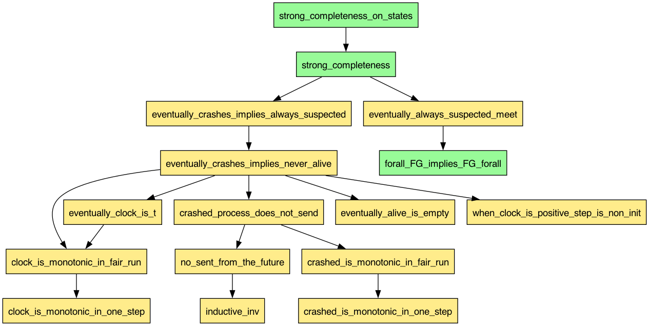
Below is the nice diagram that illustrates the dependencies between the theorems (green) and lemmas (yellow) that I had to prove, culminating in the theorem strong_completeness_on_states. Notice forall_FG_implies_FG_forall is not a lemma. Actually, it is a general theorem about swapping universal quantifiers and eventually-always, which could be reused in other proofs. Once I realized that I had to apply this lemma twice in the proof of eventually_always_suspected_meet, I finished the proof quickly. This is one more instance of that temporal logic helps us with high-level reasoning.

Surprisingly, even though strong completeness is usually thought of as a safety counterpart of strong accuracy, the proof required quite a bit of reasoning about temporal properties, not just state invariants. It also helped me a lot to structure the proofs in terms of temporal formulas, rather than in terms of arbitrary properties of computations. Of course, it would be interesting to see how this proof compares to a proof in TLAPS, which is specifically designed to reason about temporal properties.

If you look at how the lemma statements are written in Section 3, you will see that they are all temporal formulas, just written directly using quantifiers $\forall$ and $\exists$ instead of modal operators like $\square$ and $\Diamond$. To emphasize this similarity, I wrote alternative statements in TLA⁺. If you know temporal logic or TLA⁺, just have a look at all these statements:

\[\begin{align} \square (\forall m \in sent: m.ts \le clock) & \\ \square (p \notin crashed) \Rightarrow& \square \Diamond (alive[p] = \emptyset) \\ \square (p \notin crashed) \land \Diamond (q \in crashed) \Rightarrow& \Diamond \square (q \notin alive[p]) \\ \square (p \notin crashed) \land \Diamond (q \in crashed) \Rightarrow& \Diamond \square (q \in suspected[p]) \\ \square (\forall c \in \mathbb{N}: (q \in crashed \land clock = c) \Rightarrow& \square (\forall m \in sent: (m.src = q) \Rightarrow m.ts \le c)) \end{align}\]

Although a time investment of about a week to prove strong completeness of EPFD may seem like a lot, this approach has certain benefits in comparison to using tools like the explicit-state model checker TLC or the symbolic model checker Apalache:

1. Re-checking the proofs takes seconds. It’s also trivial to integrate proof-checking in the GitHub continuous integration.

2. All tools require a spec to be massaged a bit. I always felt bad about not being able to formally show that these transformations are sound with a model checker. With Lean, it is usually easy.

3. If you manage to decompose your proof goals into smaller lemmas, there is a sense of progress. Even though I had to prove 4-5 unexpected lemmas in this experiment, I could definitely say whether I was making progress or not. In the end, I only proved one lemma that happened to be redundant. With model checkers, both explicit and symbolic, it is often frustrating to wait for hours or days without clear progress.

Obviously, the downside of using an interactive theorem prover is that someone has to write the proofs. For a customer, it may make a difference whether they pay for 2–4 weeks of contract work, or for 1 week of contract work and then wait 3 weeks for a model checker. However, if time is critical, it makes sense to invest in both approaches.

Table of contents

• 1. Eventually perfect failure detector in pseudo-code
• 2. Eventually perfect failure detector in Lean
  • 2.1. Basic type definitions
  • 2.2. Partial synchrony
  • 2.3. Specifying the actions
  • 2.4. Specifying the temporal properties
  • 2.5. Specifying fairness and fair runs
• 3. Proving strong completeness in Lean
  • 3.1. Shorthand temporal definitions
  • 3.2. Warming up with simple temporal lemmas
  • 3.3. Proving completeness for two processes
    • 3.3.1. Main lemma: Eventually q is always suspected by p
    • 3.3.2. Eventually q is never alive for p
    • 3.3.3. Non-crashing p resets alive infinitely often
    • 3.3.4. A crashed process q stops sending messages
    • 3.3.5. No message sent from the future
    • 3.3.6. Other lemmas
  • 3.4. From 2 to N processes
    • 3.4.1. Defining the crashed processes
    • 3.4.2. Where do the suspected sets meet?

1. Eventually perfect failure detector in pseudo-code

To avoid any potential copyright issues, I am not copying the pseudo-code from the book. If you want to see the original version, go check DP2011¹, Algorithm 2.7, p. 55. Below is an adapted version, which simplifies the events, as we do not have to reason about the interactions between different protocol layers in the proof. Every process $p \in \mathit{Procs}$ works as follows:

upon Init do
  alive := Procs
  suspected := ∅
  delay := InitDelay
  set_timeout(delay)

upon Timeout do
  if alive ∩ suspected ≠ ∅ then
    delay := delay + InitDelay
  suspected := Procs \ alive
  send HeartbeatRequest to all p ∈ Procs
  alive := ∅
  set_timeout(delay)

upon receive HeartbeatRequest from q do
  send HeartbeatReply to q

upon receive HeartbeatReply from p do
  alive := alive ∪ {p}

Intuitively, the operation of a failure detector is very simple. Initially, a process $p$ considers all the processes alive and suspects no other process of being crashed. Also, it sets a timer to $\mathit{InitDelay}$ time units. Basically, nothing interesting happens in the time interval $[0, \mathit{InitDelay})$, except that some processes may crash.

Once a timeout is triggered on a process $p$, it updates the set of the suspected processes to the set of processes that have not sent a heartbeat to it in the previous time interval (not alive), resets the set of the alive processes and sends heartbeat requests to every process, including itself. Additionally, if $p$ finds out that it prematurely suspected an alive process, it increases its timeout window by $\mathit{InitDelay}$. Importantly, $p$ also sets a new timeout for $delay$ time units.

Finally, whenever a process receives a heartbeat request, it sends a reply. Whenever, a process receives a heartbeat reply from a process $q$, it adds $q$ to the set of alive processes.

The algorithm looks deceivingly simple. However, the pseudo-code is missing another piece of information, namely, how the distributed system behaves as a whole. What does it mean for processes to crash? When messages are received, if at all? It’s not even clear how to properly write this in pseudo-code. Normally, academic papers leave this part to math definitions. Since we want to prove correctness, we cannot avoid reasoning about the whole system. Instead of appealing to intuition, we capture both the process behavior and the system behavior in Lean.

2. Eventually perfect failure detector in Lean

In contrast to two-phase commit, where we started with a functional specification, I decided to start with the propositional specification immediately. A functional specification would be closer to the implementation details. Perhaps, we will write one in another blog post.

2.1. Basic type definitions

Before specifying the behavior of the processes, we have to figure out the basic types. You can find them in Basic.lean. First, we declare the type Proc that we use for process identities:

variable (Proc : Type) [Fintype Proc] [DecidableEq Proc] [Hashable Proc] [Repr Proc]

If you compare it with the type RM in two-phase commit, this time, we require Proc to be of Fintype. By doing so, we avoid carrying around the set of all processes. With Fintype, we can simply use Fintype.univ for the set of all processes!

Next, we define the types of message tags and messages:

/-- A message tag: `HeartbeatRequest` or `HeartbeatReply`. -/
inductive MsgTag where
  | HeartbeatRequest
  | HeartbeatReply
  deriving DecidableEq, Repr

/-- A message that is sent by one process (src) to another process (dst).
    Every message is equipped with a timestamp, which is equal to the
    clock value at the time of sending the message.
 -/
@[ext]
structure Msg where
  kind: MsgTag
  src: Proc
  dst: Proc
  timestamp: ℕ
  deriving DecidableEq, Repr

Now, most of it should be obvious, except, perhaps, for the field timestamp. What is it? If we look at the original paper on failure detectors by Chandra and Toueg (CT96), we’ll see that they assume the existence of a global clock. The processes can’t read this clock, but the system definitions refer to it. Hence, a message’s timestamp refers to the value of the global clock at the moment the message is sent.

Finally, we define a protocol state with the following structure:

structure ProtocolState where
  alive: Std.HashMap Proc (Finset Proc)
  suspected: Std.HashMap Proc (Finset Proc)
  delay: Std.HashMap Proc Nat
  nextTimeout: Std.HashMap Proc Nat
  sent: Finset (Msg Proc)
  rcvd: Finset (Msg Proc)
  clock: Nat
  crashed: Finset Proc

The first group of fields should be clear. They map process identities to the corresponding values of the variables in the pseudo-code:

• alive[p]! stores the set of alive processes as observed by a process p,
• suspected[p]! stores the set of suspected processes as observed by a process p,
• delay[p]! stores the current value of delay by a process p,
• nextTimeout[p]! stores the timestamp of the next timeout by a process p. The timestamp refers to the global clock.

The second group of fields is less obvious. They do not represent the process states, but rather the rest of the global state of the distributed system:

• sent is the set of all messages sent by the processes,
• rcvd is the set of all messages received by the processes,
• clock is the value of the fictitious global clock,
• crashed is the set of all processes that have crashed.

While the second group of fields is needed to formally capture a state of the distributed system, we notice that the processes cannot have access to those fields. Otherwise, detecting failures would be trivial, we would just access the field crashed.

If you find this representation of the global state surprising, it’s actually quite common to reason about such a global snapshot of a distributed system in TLA⁺. Here, we’re simply following the TLA⁺ methodology, albeit reproduced in Lean.

2.2. Partial synchrony

The algorithm is designed to work under partial synchrony. Unfortunately, DP2011 does not give us a precise definition of what this means. So we go back to the paper by Dwork, Lynch, and Stockmeyer (DLS88) who introduced partial synchrony. There are several kinds of partial synchrony in the paper. We choose the one that is probably the most commonly used nowadays: There is a period of time called global stabilization time (GST), after which every correct process $p$ receives a message from a correct process $q$ no later than $\mathit{MsgDelay}$ time units after it was sent by $q$. Both $\mathit{GST}$ and $\mathit{MsgDelay}$ are unknown to the processes, and may change from run to run. It is also important to fix the guarantees about the messages that were sent before $\mathit{GST}$. We assume that they are received by $\mathit{GST} + \mathit{MsgDelay}$ the latest.

Now we can write a formal definition of what it means for a message to be received on time under partial synchrony:

/--
  Given a message that was sent at `timestamp`, can a process receive it at time `clock`.
  -/
def isMsgTimely (GST: Nat) (MsgDelay: Nat) (timestamp: Nat) (clock: Nat): Bool :=
  clock ≥ timestamp && clock ≤ (max GST timestamp) + MsgDelay

Both DLS88 and DP2011 mention that in practice partial synchrony means that the periods of asynchrony and synchrony alternate. DLS88 mention that for their consensus algorithms one should be able to compute the time of convergence after GST. I am not actually sure how it would work in case of failure detectors, as it is impossible to predict how long it takes a process to crash. Hence, in our model, there is no alternation of asynchrony and synchrony. After GST, communication becomes synchronous, in the sense that every message is delivered not later than $\mathit{MsgDelay}$ time units after it was sent.

2.3. Specifying the actions

Now we are ready to specify the actions of a distributed system that follows the algorithm. You can find all definitions in Propositional.lean.

We start with the protocol parameters and the variables s and s' that we use throughout the definitions:

-- The abstract type of processes
variable (Proc : Type) [Fintype Proc] [DecidableEq Proc] [Hashable Proc] [Repr Proc]

-- The initial delay Δ used by the processes
variable (InitDelay: ℕ)

-- The global stabilization time GST, unknown to the processes
variable (GST: ℕ)

-- The message delay after GST, unknown to the processes
variable (MsgDelay: ℕ)

-- The state `s` is a state of the protocol, explicitly added to all the functions.
variable (s: ProtocolState Proc)

-- The state `s'` is the "next" state of the protocol.
variable (s': ProtocolState Proc)

Below is the definition of receiving a heartbeat request:

/--
  A process `dst` receives a heartbeat request from `src`.
  -/
def rcv_heartbeat_request (src: Proc) (dst: Proc) (timestamp: ℕ) :=
  let req := { kind := MsgTag.HeartbeatRequest, src, dst, timestamp }
  dst ∉ s.crashed
  ∧ req ∈ s.sent
  ∧ isMsgTimely GST MsgDelay timestamp s.clock
  ∧ s'.rcvd = s.rcvd ∪ { req }
  ∧ let reply :=
      { kind := MsgTag.HeartbeatReply, src := dst, dst := src, timestamp := s.clock }
    s'.sent = s.sent ∪ { reply }
  ∧ s'.crashed = s.crashed
  ∧ s'.clock = s.clock
  ∧ s'.alive = s.alive
  ∧ s'.suspected = s.suspected
  ∧ s'.delay = s.delay
  ∧ s'.nextTimeout = s.nextTimeout

As you can see, the definition of rcv_heartbeat_request captures the behavior of the whole system, when dst handles a heartbeat request. In particular, dst cannot be in the crashed state when it is receiving the message, the message has to be timely, etc. Similar to TLA⁺, we specify that certain fields preserve their values. Actually, we could update the structure s' instead of writing down multiple equalities over the fields. However, it would make the proofs more cumbersome. I could not find a simple way to express something like TLA⁺’s UNCHANGED over multiple variables.

Interestingly, I accidentally swapped src and dst in the initial version of reply in rcv_heartbeat_request. I only found that when trying to prove one of the lemmas towards strong completeness.

Similar to rcv_heartbeat_request, we specify rcv_heartbeat_reply:

/--
  A process `dst` receives a heartbeat reply from `src`.
  -/
def rcv_heartbeat_reply (src: Proc) (dst: Proc) (timestamp: ℕ) :=
  let reply := { kind := MsgTag.HeartbeatReply, src, dst, timestamp }
  dst ∉ s.crashed
  ∧ reply ∈ s.sent
  ∧ isMsgTimely GST MsgDelay timestamp s.clock
  ∧ s'.rcvd = s.rcvd ∪ { reply }
  ∧ let nextAlive := s.alive[dst]! ∪ { src }
    s'.alive = s.alive.insert dst nextAlive
  ∧ s'.sent = s.sent
  ∧ s'.crashed = s.crashed
  ∧ s'.clock = s.clock
  ∧ s'.suspected = s.suspected
  ∧ s'.delay = s.delay
  ∧ s'.nextTimeout = s.nextTimeout

The definition of timeout is the longest one, as a lot of things happen on timeout:

/--
  A process `p` timeouts.
  -/
def timeout (p: Proc) :=
    p ∉ s.crashed
  ∧ s.clock = s.nextTimeout[p]!
  -- if `p` suspects an alive process, increase the delay
  ∧ let nextDelay :=
      if s.alive[p]! ∩ s.suspected[p]! ≠ ∅
      then s.delay[p]! + InitDelay
      else s.delay[p]!
    s'.delay = s.delay.insert p nextDelay
  -- recompute the set of suspected processes
  ∧ let nextSuspected := Finset.univ \ s.alive[p]!
      /- q ∉ s.alive[p]! is equivalent to the original code:
        on q ∉ s.alive[p]! ∧ q ∉ s.suspected[p]! trigger Suspect q
        on q ∈ s.alive[p]! ∧ q ∈ s.suspected[p]! trigger Restore q
        else keep q ∈ s.suspected[p]!
       -/
    s'.suspected = s.suspected.insert p nextSuspected
  -- send heartbeat requests to all processes, including `p` itself
  ∧ s'.sent = s.sent ∪ Finset.univ.image (fun q => {
      kind := MsgTag.HeartbeatRequest, src := p, dst := q, timestamp := s.clock
    })
  -- set alive to empty and reset the timer
  ∧ s'.alive = s.alive.insert p ∅
  ∧ s'.nextTimeout = s.nextTimeout.insert p (s.clock + s.delay[p]!)
  -- everything else remains unchanged
  ∧ s'.rcvd = s.rcvd
  ∧ s'.crashed = s.crashed
  ∧ s'.clock = s.clock

As you can see, the sequential logic from the pseudo-code is compressed into multiple equalities, very much in the spirit of TLA⁺. Our proofs are complex enough, so it’s good that we do not have to deal with sequential execution inside actions. If this is not convincing enough, we could write sequential code and prove that it refines the corresponding propositional definition.

We have defined the three actions, as in the pseudo-code (the definition of init comes later). Are we done? Not quite. Since we’re specifying the behavior of the entire distributed system, not just individual processes, we need two more actions.

The first additional action is crash:

/--
  A process `p` crashes. This action is not part of the protocol itself, but
  rather a part of the environment (or the adversary).
  -/
def crash (p: Proc) :=
    p ∉ s.crashed
  ∧ s'.crashed = s.crashed ∪ { p }
  ∧ s'.sent = s.sent
  ∧ s'.rcvd = s.rcvd
  ∧ s'.clock = s.clock
  ∧ s'.alive = s.alive
  ∧ s'.suspected = s.suspected
  ∧ s'.delay = s.delay
  ∧ s'.nextTimeout = s.nextTimeout

Yes, we have to specify what it means for a process to crash, as there is no built-in semantics of crashing in Lean.

What is left? Remember that we had the fictitious global clock? We have to advance it from time to time:

/--
  The global system clock advances. We advance the clock by exactly one unit.
  If we had a rational clock, we would have to advance it by `delta` units.
  -/
def advance_clock :=
    s'.clock = s.clock + 1
  ∧ s'.crashed = s.crashed
  ∧ s'.sent = s.sent
  ∧ s'.rcvd = s.rcvd
  ∧ s'.alive = s.alive
  ∧ s'.suspected = s.suspected
  ∧ s'.delay = s.delay
  ∧ s'.nextTimeout = s.nextTimeout

I have cut a corner in the definition of advance_clock by incrementing it, instead of advancing it by a positive delta. This works since we declared the clock to be a natural number rather than a rational or real. Incrementing the clock instead of advancing it by delta simplifies the proofs a bit.

Finally, we define the initialization and the transition relation as follows:

/--
  Initialize a map with the default value `v` for each process in `all`.
  -/
noncomputable def init_map {α: Type} (v: α) : Std.HashMap Proc α :=
  Finset.univ.toList.foldl (fun m p => m.insert p v) (Std.HashMap.emptyWithCapacity 0)

/--
  The initial state of the protocol.
  -/
def init: Prop :=
    s.crashed = ∅
  ∧ s.sent = ∅
  ∧ s.rcvd = ∅
  ∧ s.clock = 0
  ∧ s.alive = init_map Proc ∅
  ∧ s.suspected = init_map Proc ∅
  ∧ s.delay = init_map Proc InitDelay
  ∧ s.nextTimeout = init_map Proc InitDelay

/--
  The transition relation of the protocol.
  -/
def next: Prop :=
    advance_clock Proc s s'
  ∨ ∃ p: Proc,
        timeout Proc InitDelay s s' p
      ∨ crash Proc s s' p
      ∨ ∃ q: Proc, ∃ t: ℕ,
            rcv_heartbeat_request Proc GST MsgDelay s s' p q t
          ∨ rcv_heartbeat_reply Proc GST MsgDelay s s' p q t

Notice the noncomputable qualifier in front of init_map. Lean requires it, as we are converting Finset.univ to a list. If we want to write an executable specification, we have to work around this, perhaps, by passing the list of all process identities to the initializer.

So far, our definitions looked very much like a typical specification in TLA⁺, even though we had to use Lean’s data structures such as finite sets and hash maps, instead of TLA⁺’s sets and functions. I believe that there is an advantage in keeping this resemblance. First, if we choose to translate this specification to TLA⁺, e.g., to use the model checkers, it is not hard. (Actually, I did that; it was almost no-brainer with Copilot). Second, we can reuse the standard specification idioms from TLA⁺.

2.4. Specifying the temporal properties

In two-phase commit, we were only concerned with state invariants and, thus, only had to reason about lists of actions. In the case of failure detectors, we have to reason about temporal properties. In general, temporal properties require us to reason about infinite behaviors. Surprisingly, it is quite easy to specify properties of infinite behaviors in Lean. We just use a function seq of natural numbers to ProtocolState.

Here is how we specify strong completeness of the failure detector:

def is_strongly_complete
    (Crashed: Finset Proc)
    (seq: ℕ → ProtocolState Proc): Prop :=
  (∀ p: Proc, p ∈ Crashed ↔ ∃ i: ℕ, p ∈ (seq i).crashed)
    → ∃ k: ℕ,
        ∀ i: ℕ,
          ∀ p q: Proc,
            p ∉ Crashed ∧ q ∈ Crashed → q ∈ (seq (k + i)).suspected[p]!

The above definition may seem to be a bit loaded. The left part of → requires that the set Crashed indeed contains all the processes that crashed in the run. The set Crashed happened to be hard to define. More on that later. The right part of → says that there is a point k in seq, so that starting with $k$, every further state $seq (i + k)$ satisfies $q \notin (seq (i + k)).suspected[p]!$ for a correct $p$ and a crashed $q$.

If you know temporal logic, e.g., as defined in TLA⁺, the right-hand side of → could be written like (<> is usually called “eventually” and [] is called “always”):

<>[](∀ p q: Proc, p ∉ C ∧ q ∈ C → q ∈ suspected[p])

Similar to is_strongly_complete, this is how we specify strong accuracy:

def is_eventually_strongly_accurate
    (Crashed: Finset Proc)
    (seq: ℕ → (ProtocolState Proc)) : Prop :=
  (∀ p: Proc, p ∈ Crashed ↔ ∃ i: ℕ, p ∈ (seq i).crashed)
    → ∃ k: ℕ,
        ∀ i: ℕ,
          ∀ p q: Proc,
            p ∉ Crashed ∧ q ∉ Crashed → q ∉ (seq (i + k)).suspected[p]!

Again, in temporal logic it would look like:

<>[](∀ p q: Proc, p ∉ crashed ∧ q ∉ crashed → q ∉ suspected[p])

Don’t we need a framework for temporal logic? Well, actually not. Instead of [] and <>, we can simply use ∀ and ∃ over indices. There is even a deeper connection between linear temporal logic and first-order logic with ordering, shown by Hans Kamp. For example, see a recent Proof of Kamp’s theorem by Alexander Rabinovich. Temporal formulas are often easier to read. So I prefer to accompany properties in Lean with temporal properties in the documentation.

2.5. Specifying fairness and fair runs

Now that we have described the system behavior, can we proceed with the proofs? Not so fast. If you have ever tried to prove liveness, you know that we have to restrict our analysis to fair system executions.

For instance, our definition of next allows the scheduler to always choose advance_clock as the next action. So we would end up with a sequence that consists of states that only have the increasing clock values. Is it an interesting sequence? Not really. We have not even had a chance to try other actions. Usually, such executions are called unfair. We want to restrict our liveness analysis to fair executions.

To save you guess work, here are the three kinds of conditions we want from a fair execution in our failure detector:

1. For every message $m$ that is sent, the message destination receives it on time, unless it crashes before the message $m$ expires. This is the constraint right from partial synchrony.

2. If a process $p$ has a scheduled timeout, $p$ should process the timeout before the global clock advances too far, unless $p$ crashed before the timeout had to be handled. While this may sound obvious, this requirement is crucial for the failure detector.

3. The global clock must advance infinitely often. Indeed, it is possible to construct a sequence of states that have the global clock increased only finitely many times. This effect is usually called zenoness, after Zeno’s paradoxes. We want to avoid such executions. If you do not believe this is possible, look carefully at the definition rcv_heartbeat_request. It can receive the same message multiple times! Sure, we could eliminate this behavior by receiving every message at most once. It would be harder to do that in a more complex protocol. Just requiring non-zenoness is much simpler.

Lean has no idea about distributed algorithms and fair executions. We can get some inspiration from TLA⁺. Unfortunately, fairness in TLA⁺ is a bit too complicated. If we wanted to transfer this approach to our proofs, we would have to figure out how to write our fairness constraints with strong fairness, weak fairness, and ENABLED.

To avoid this complex ceremony, we recall that our actions have very simple structure. Essentially, every protocol state is constructed by executing one of the six actions:

inductive Action where
  | Init
  | AdvanceClock
  | Timeout(p: Proc)
  | Crash(p: Proc)
  | RcvHeartbeatRequest(src: Proc) (dst: Proc) (timestamp: ℕ)
  | RcvHeartbeatReply(src: Proc) (dst: Proc) (timestamp: ℕ)

Our key idea here is that we could explicitly force some of the actions to be taken in a fair execution. To this end, we refine our transition relation next with next_a:

def next_a (a: @Action Proc): Prop :=
match a with
| Action.Init =>
    s' = s -- dummy action
| Action.AdvanceClock =>
    advance_clock Proc s s'
| Action.Timeout p =>
    timeout Proc InitDelay s s' p
| Action.Crash p =>
    crash Proc s s' p
| Action.RcvHeartbeatRequest src dst timestamp =>
    rcv_heartbeat_request Proc GST MsgDelay s s' src dst timestamp
| Action.RcvHeartbeatReply src dst timestamp =>
    rcv_heartbeat_reply Proc GST MsgDelay s s' src dst timestamp

Of course, we would have to prove equivalence of next and next_a. Actually, we have to account for the case Init, where we just require $s’ = s$. This is easy to do in Lean. Below is the theorem statement. Check PropositionalProofs.lean for the actual proof:

theorem next_a_iff_next
    (s: ProtocolState Proc)
    (s': ProtocolState Proc):
      s' = s ∨ next Proc InitDelay GST MsgDelay s s'
        ↔ ∃ a: Action Proc, next_a Proc InitDelay GST MsgDelay s s' a := by

Now, instead of reasoning just about sequences of protocol states, we can reason about sequences of states and actions. Formally, we introduce the definition of a trace and related definitions:

structure StateAction where
  s: ProtocolState Proc
  a: @Action Proc

/--
  A trace is an infinite sequence of pairs:
   - a state and
   - the action that produced the state from the previous one.

  The initial state is produced by the dummy action `Init`.
  We do not enforce the states to be connected by the `next` relation.
  See `is_path` and `is_run` for stronger conditions.
  -/
abbrev Trace := ℕ → StateAction Proc

/--
  Interpret a trace as a sequence of protocol states.
  -/
def states_of_trace (tr: Trace Proc) :=
  fun i: ℕ => (tr i).s

Not every trace can be produced by the failure detector protocol. We define what it means for a trace to be a run of the protocol, not necessarily a fair one, and what it means for a trace to be a fair run of the protocol:

/--
  A trace is a path, if every pair of state-action pairs `((s_i, _), (s_{i+1},
  a_{i+1})` is a transition via `next_a`. A path does not have to start with an
  initial state.
  -/
def is_path (tr: Trace Proc) : Prop :=
  ∀ i: ℕ,
    next_a Proc InitDelay GST MsgDelay (tr i).s (tr (i + 1)).s (tr (i + 1)).a

/--
  A trace is a (protocol) run, if it starts with an initial state,
  and it is a path.
  -/
def is_run (tr: Trace Proc) : Prop :=
  let s0 := (tr 0).s
  init Proc InitDelay s0
    ∧ is_path Proc InitDelay GST MsgDelay tr

/--
  Does a trace constitute a fair run of the protocol?
  -/
def is_fair_run (tr: Trace Proc) : Prop :=
  is_run Proc InitDelay GST MsgDelay tr
    ∧ is_reliable_communication Proc GST MsgDelay tr
    ∧ is_fair_timeout Proc tr
    ∧ is_fair_clock Proc tr

Having all these definitions, we proceed with our fairness constraints. The simplest one is is_fair_clock:

def is_fair_clock (tr: Trace Proc) : Prop :=
  ∀ i: ℕ,
    ∃ j: ℕ,
      j > i ∧ (tr j).a = Action.AdvanceClock

Essentially, is_fair_clock says that we observe AdvanceClock in a trace infinitely often. In TLA⁺, it would be written like <>[]<advance_clock>_vars. If you don’t know what it means, just skip it.

Further, we define is_fair_timeout as follows:

def is_fair_timeout (tr: Trace Proc): Prop :=
  ∀ i: ℕ,
    ∀ p: Proc,
      ∃ k: ℕ,
        (p ∉ (tr (i + k - 1)).s.crashed → (tr (i + k)).a = Action.Timeout p)
          -- TODO: is this a bit too strong in the presence of is_fair_clock?
          ∧ (tr (i + k)).s.clock = (tr i).s.nextTimeout[p]!

Finally, is_reliable_communication has the longest definition:

def is_reliable_communication (tr: Trace Proc) : Prop :=
  ∀ k: ℕ,
    ∀ m ∈ (tr k).s.sent,
      ∃ i: ℕ,
        let { s := s_j, a := a_j } := tr (k + i)
        isMsgTimely GST MsgDelay m.timestamp s_j.clock
          ∧ m.dst ∈ s_j.crashed
            ∨ match m.kind with
            | MsgTag.HeartbeatReply =>
                a_j = Action.RcvHeartbeatReply m.src m.dst m.timestamp
            | MsgTag.HeartbeatRequest =>
                a_j = Action.RcvHeartbeatRequest m.src m.dst m.timestamp

Now we are ready for the proofs!

3. Proving strong completeness in Lean

The main theorem that we want to prove is strong_completeness_on_states, which basically delegates the work to strong_completeness over fair traces:

/--
  Show that the property `is_strongly_complete` holds on fair runs.
  -/
theorem strong_completeness_on_states
    (tr: Trace Proc)
    (h_is_fair_run: is_fair_run Proc InitDelay GST MsgDelay tr)
    (Crashed: Finset Proc):
      is_strongly_complete Proc Crashed (states_of_trace Proc tr) := by
  unfold is_strongly_complete states_of_trace
  intro h_crashed
  have h_is_crashing_set: is_crashing_set tr Crashed := by exact h_crashed
  exact strong_completeness InitDelay GST MsgDelay
    tr h_is_fair_run Crashed h_is_crashing_set

The below figure summarizes the lemmas (yellow) and theorems (green) that I had to prove, in order to show strong_completeness_on_states.

If you want to understand the proofs, you should inspect PropositionalProofs.lean with the Lean extension for VSCode. I will only give you human-readable summaries as well as my observations about how I wrote these proofs.

3.1. Shorthand temporal definitions

I found it convenient to define shorthands for the temporal properties that are used throughout the proofs. For instance, below is the definition of never_crashes:

/-- A process `p` never crashes, i.e., `[](p ∉ crashed)`.  -/
def never_crashes (tr: Trace Proc) (p: Proc): Prop :=
  ∀ i: ℕ,
    p ∉ (tr i).s.crashed

This property can be visualized as follows:

Time →	0	1	2	3	4	5
crashed:	{}	{}	{}	{}	{}	{}
	✅	✅	✅	✅	✅	✅

[](p ∉ crashed) holds

The negation of never_crashes is eventually_crashes:

/-- A process `p` eventually crashes, i.e., `<>(p ∈ crashed)`.  -/
def eventually_crashes (tr: Trace Proc) (p: Proc): Prop :=
  ∃ i: ℕ,
    p ∈ (tr i).s.crashed

Time →	0	1	2	3	4	5
crashed:	{}	{}	{}	{p}	{p}	{p}
	❌	❌	❌	✅	✅	✅

<>(p ∈ crashed) holds

We also need eventually_never_alive:

/--
  Eventually, `p` never registers `q` as alive, i.e., `<>[](q ∉ alive[p])`.
  -/
def eventually_never_alive (tr: Trace Proc) (p q: Proc): Prop :=
  ∃ k: ℕ, ∀ i: ℕ,
    q ∉ (tr (k + i)).s.alive[p]!

Time →	0	1	2	3	4	5
alive[p]:	{q}	{q}	{q}	{}	{}	{}
	❌	❌	❌	✅	✅	✅

<>[] (q ∉ alive[p]) holds

We also need q_is_always_suspected and eventually_q_is_always_suspected:

/--
  `p` suspects `q` permanently from some point `k`, i.e.,
  `tr[k,...] ⊧ [](q ∈ suspected[p])`.
  -/
def q_is_always_suspected (tr: Trace Proc) (p q: Proc) (k: ℕ): Prop :=
  ∀ i: ℕ,
    q ∈ (tr (k + i)).s.suspected[p]!

/--
  Eventually, `p` suspects `q` permanently, i.e., `<>[](q ∈ suspected[p])`.
  -/
def eventually_q_is_always_suspected (tr: Trace Proc) (p q: Proc): Prop :=
  ∃ k: ℕ,
    q_is_always_suspected tr p q k

Time →	0	1	2	3	4	5
suspected[p]:	{}	{}	{}	{q}	{q}	{q}
	❌	❌	❌	✅	✅	✅

<>[] (q ∈ suspected[p]) holds

Finally, we need the definition of the set of crashing processes:

/--
  A set of processes `C` is a crashing set if every process in `C`
  eventually crashes, and every process not in `C` never crashes.
 -/
def is_crashing_set (tr: Trace Proc) (C: Finset Proc): Prop :=
  ∀ p: Proc, p ∈ C ↔ eventually_crashes tr p

3.2. Warming up with simple temporal lemmas

Before discussing hard-to-prove lemmas, let’s have a look at a few very simple ones. To start with, we can easily show that the global clock never decreases in a single step. The proof is basically done by the simp tactic:

/--
  A single step does not decrease the clock value. In temporal logic,
  `[](clock' ≥ clock)`.
  -/
lemma clock_is_monotonic_in_one_step
    (s: ProtocolState Proc) (s': ProtocolState Proc) (a: Action Proc)
    (h_next: next_a Proc InitDelay GST MsgDelay s s' a):
      s'.clock ≥ s.clock := by
  unfold next_a crash rcv_heartbeat_reply advance_clock
         rcv_heartbeat_request timeout at h_next
  cases a with
  | Init => simp at h_next; rw [h_next]
  | AdvanceClock | RcvHeartbeatRequest _ _ _
  | RcvHeartbeatReply _ _ _ | Timeout _ | Crash _ =>
    simp [h_next]

Very much similar to clock_is_monotonic_in_one_step, we can prove that the set of the crashed processes can only grow in a single step:

/--
  A single step does not decrease the set of the crashed processes.
  In temporal logic, `[](crashed' ⊇ crashed)`.
  -/
lemma crashed_is_monotonic_in_one_step
    (s: ProtocolState Proc) (s': ProtocolState Proc) (a: Action Proc)
    (h_next: next_a Proc InitDelay GST MsgDelay s s' a):
      s'.crashed ⊇ s.crashed := by
  -- literally the same proof as above
  unfold next_a crash rcv_heartbeat_reply
         advance_clock rcv_heartbeat_request timeout at h_next
  cases a with
  | Init => simp at h_next; rw [h_next]
  | AdvanceClock | RcvHeartbeatRequest _ _ _
  | RcvHeartbeatReply _ _ _ | Timeout _ | Crash _ =>
    simp [h_next]

We use these simple lemmas to prove that $clock$ never decreases in a fair run, and once a process has crashed, it always remains crashed. In both cases, the proof is done by simple induction over the indices in a fair run. For example, here is the lemma crashed_is_monotonic_in_fair_run, together with its proof:

/--
  The set `crashed` grows monotonically in a fair run.

  In temporal logic, `∀p: Proc, [](p ∈ crashed) → [](p ∈ crashed))`.
  -/
lemma crashed_is_monotonic_in_fair_run
    (tr: Trace Proc)
    (h_is_fair_run: is_fair_run Proc InitDelay GST MsgDelay tr)
    (p: Proc) (k: ℕ) (h_p_crashed: p ∈ (tr k).s.crashed) (i: ℕ):
      p ∈ (tr (k + i)).s.crashed := by
  induction i with
  | zero => exact h_p_crashed
  | succ i ih =>
    unfold is_fair_run at h_is_fair_run
    rcases h_is_fair_run with ⟨ h_is_run, _ ⟩
    unfold is_run at h_is_run
    rcases h_is_run with ⟨ _, h_is_path ⟩
    unfold is_path at h_is_path
    specialize h_is_path (k + i)
    -- apply crashed_is_monotonic_in_one_step to the last step
    have h_last_step_mono :=
      crashed_is_monotonic_in_one_step InitDelay GST MsgDelay
        (tr (k + i)).s (tr (k + i + 1)).s (tr (k + i + 1)).a h_is_path
    exact h_last_step_mono ih

Further, we prove another useful lemma: Given a clock value $t$, eventually the global clock reaches the value $t$:

/--
  Every fair run covers every clock value `t`. Note that this requires fairness.
  Otherwise, the clock may not advance at all.

  In temporal logic, `∀t ∈ ℕ, <>(clock ≥ t)`.
  -/
lemma eventually_clock_is_t
    (tr: Trace Proc)
    (h_is_fair_run: is_fair_run Proc InitDelay GST MsgDelay tr)
    (t: ℕ):
      (∃ i: ℕ, (tr i).s.clock ≥ t) := by

You can check the full proof of eventually_clock_is_t. It is not a long one, but it requires a bit of linear arithmetic to reason about indices and clock constraints.

3.3. Proving completeness for two processes

Before we dive into the results for all processes, we focus on just two processes in a fair run tr:

• a process p that never crashes in tr,
• a process q that eventually crashes in tr.

Since the Lean proofs are quite detailed, I provide the lemmas with short human-readable proofs. Actually, I had to write proof schemas on paper, before developing detailed proofs. The math-like proofs below are summaries of the detailed Lean proofs, as my pen & paper proofs had several flaws.

3.3.1. Main lemma: Eventually q is always suspected by p

To show strong completeness for $p$ and $q$, we prove the following key lemma:

Lemma eventually_crashes_implies_always_suspected. If $q$ crashes at some time $j$ and $p$ never crashes, then there exists $k$ such that for all $i \ge k$, we have $q \in \text{suspected}[p]$ at $i$.

Using the TLA⁺ notation, we could write this lemma in temporal logic:

\[\square (p \notin crashed) \land \Diamond (q \in crashed) \Rightarrow \Diamond \square (q \in suspected[p])\]

This is how the lemma is formulated in Lean:

lemma eventually_crashes_implies_always_suspected
    (tr: Trace Proc)
    (h_is_fair_run: is_fair_run Proc InitDelay GST MsgDelay tr)
    (p q: Proc)
    (h_p_never_crashes: never_crashes tr p)
    (h_crashes: eventually_crashes tr q):
      eventually_q_is_always_suspected tr p q := by

You can check the detailed proof in Lean. The proof is about 100 LOC long. I have asked ChatGPT to summarize the proof similar to a mathematician’s proof. It looked very convincing, but the AI has hallucinated a lot, by inventing additional lemmas and mixing process names. Instead, here is my proof summary, 100% organic:

Proof. Since $q$ eventually crashes, we apply Lemma eventually_crashes_implies_never_alive (see below) to show that there is an index $k$ such that for all $i \ge k$, we have $q \notin alive[p]$ at $i$. Now, we may still have $q \in suspected[p]$ at $k$. Hence, we apply the fairness constraint is_fair_timeout to show that there is an index $j > k$ such that $p$ timeouts at $j$. By the definition of timeout, we have $q \in suspected[p]$ at $j + 1$, as the action timeout updates suspected[p] with Finset.univ \ alive[p], and $q \notin alive[p]$ at $j$.

It remains to show that $q \in suspected[p]$ at an arbitrary $i > j$. We do this by induction on $i$. All actions except Timeout preserve the value of the field suspected, so we have $q \in suspected[p]$. In case of Timeout r, we consider two cases: (1) $r \ne p$, and (2) $r = p$. When $r \ne p$, the value of $suspected[p]$ does not change. When $r = p$, we again invoke the conclusion that $q \notin alive[p]$ at $i$. Similar to the above reasoning about the action timeout, we conclude $q \in suspected[p]$ at all $i > j$. $\blacksquare$

3.3.2. Eventually q is never alive for p

As you have noticed, we invoked Lemma eventually_crashes_implies_never_alive. This is how it looks like in a human-readable form:

Lemma eventually_crashes_implies_never_alive. If $q$ crashes at some time $j$ and $p$ never crashes, then there exists $k$ such that for all $i \ge k$, we have $q \notin \text{alive}[p]$ at $i$.

Using the TLA⁺ notation, we could write this lemma in temporal logic:

\[\square (p \notin crashed) \land \Diamond (q \in crashed) \Rightarrow \Diamond \square (q \notin alive[p])\]

This is how the lemma is formulated in Lean, the detailed proof in Lean is 170 LOC:

lemma eventually_crashes_implies_never_alive
    (tr: Trace Proc)
    (h_is_fair_run: is_fair_run Proc InitDelay GST MsgDelay tr)
    (p q: Proc)
    (h_p_never_crashes: never_crashes tr p)
    (h_crashes: eventually_crashes tr q):
      eventually_never_alive tr p q := by

Proof. Since $q$ eventually crashes, there is an index $i_{crash}$, so $q \in crashed$ at $i_{crash}$. Let’s denote with $t_{crash}$ the clock value at $i_{crash}$. However, $p$ may still receive heartbeats from $q$ that were sent in the past. Hence, we choose the time point $t_{magic}$:

\[t_{magic} = max(\mathit{GST} + \mathit{MsgDelay}, t_{crash} + \mathit{MsgDelay}) + 1\]

We invoke Lemma eventually_clock_is_t to show that eventually the global clock reaches the value $t_{magic}$. Further, we invoke Lemma eventually_alive_is_empty (see below) to show that eventually $alive[p] = \emptyset$ after that point. Hence, we have an index $i_{empty}$ with the following constraints at:

1. $alive[p] = \emptyset$ at $i_{empty}$,

2. $q$ has crashed and no heartbeats from $q$ can longer arrive, as the global clock is past $\mathit{GST} + \mathit{MsgDelay}$,

The rest of the proof goes by induction over $i \ge i_{empty}$. We have already shown the inductive base. The inductive step is proven by contradiction: Assume that there is an index $i + 1$, where $alive[p] \ne \emptyset$. We do case analysis on the action that produces the state at $i + 1$. There are two interesting cases:

1. A process $r$ times out. If $r \ne p$, the $r$ keeps the value of $alive[p]$. If $p$ times out, it resets $alive[p]$ to $\emptyset$. In both cases, $alive[p] = \emptyset$.

2. A process $\mathit{dst}$ receives a heartbeat reply $m$ from a process $\mathit{src}$. The cases of $dst \ne p$ or $src \ne q$ are trivial, as the predicate $q \in alive[p]$ does not change in those cases. The case of $src = q$ and $dst = p$ is the hardest one. First, we apply Lemma crashed_process_does_not_send (see below) to show that the message timestamp $m.ts$ is not greater than $t_{crash}$. Second, we apply Lemma clock_is_monotonic_in_fair_run to show that $clock \ge t_{magic}$ at point $i$. Third, we apply the constraint isMsgTimely from the definition of rcv_heartbeat_reply. We arrive at the following combination of linear constraints that do not have a solution:

\[\require{cases} \begin{cases} \mathit{m.ts} &\le t_{crash}\\ clock &\ge t_{magic}\\ clock &\ge m.ts\\ clock &\le max(GST, m.ts) + \mathit{MsgDelay} \end{cases}\]

This inductive argument finishes the proof. $\blacksquare$

3.3.3. Non-crashing p resets alive infinitely often

We invoked Lemma eventually_alive_is_empty in the previous section. This is how this lemma looks like in a human-readable form:

Lemma eventually_alive_is_empty. If $p$ never crashes, then for every $k > 0$, there is $i \ge k$ such that we have $\text{alive}[p] = \emptyset$ at $i$.

Using the TLA⁺ notation, we could write this lemma in temporal logic:

\[\square (p \notin crashed) \Rightarrow \square \Diamond (alive[p] = \emptyset)\]

This is how the lemma is formulated in Lean, the detailed proof in Lean is 30 LOC:

lemma eventually_alive_is_empty
    (tr: Trace Proc)
    (h_is_fair_run: is_fair_run Proc InitDelay GST MsgDelay tr)
    (p: Proc)
    (h_p_never_crashes: never_crashes tr p)
    (k: ℕ)
    (h_i_positive: k > 0):
      ∃ i: ℕ, (tr (k + i)).s.alive[p]! = ∅ := by

Proof. Since $p$ never crashes, we apply the fairness constraint is_fair_timeout to the index $k$. Hence, there exists an index $i$, so that $p$ times out at $k + i$. When processing the action timeout, process $p$ resets $alive[p]$ to the empty set. $\blacksquare$

3.3.4. A crashed process q stops sending messages

We invoked Lemma crashed_process_does_not_send in the proof of eventually_crashes_implies_never_alive. This is how this lemma looks like in a human-readable form:

Lemma crashed_process_does_not_send. If $q$ is crashed at $k$ and the clock value at $k$ equals to some $c$, then for every $i \ge 0$ and every message $m \in sent$ at $k + i$, if $m.src = q$, then $m.ts \le c$.

Using the TLA⁺ notation, we could write this lemma in temporal logic:

\[\square (\forall c \in \mathbb{N}: (q \in crashed \land clock = c) \Rightarrow \square (\forall m \in sent: (m.src = q) \Rightarrow m.ts \le c))\]

This is how the lemma is formulated in Lean, the detailed proof in Lean is 110 LOC:

lemma crashed_process_does_not_send
    (tr: Trace Proc)
    (h_is_fair_run: is_fair_run Proc InitDelay GST MsgDelay tr)
    (p: Proc) (k: ℕ) (h_p_crashed: p ∈ (tr k).s.crashed):
      ∀ i: ℕ,
        ∀ m ∈ (tr (k + i)).s.sent,
          m.src = p → m.timestamp ≤ (tr k).s.clock := by

Although this lemma seems to be obvious, the proof is relatively long. It is mostly technical.

Proof. The proof is done by induction on $i$. It invokes two other lemmas:

1. Lemma crashed_is_monotonic_in_fair_run that we discussed before, and

2. Lemma no_sent_from_the_future (see below), which states that no message can have a timestamp above the current value of the global clock.

The induction goes by case analysis on the action that is executed at point $i$. There are two interesting cases that extend the set of sent messages $sent$:

1. A timeout by process $r$. Since $q$ crashed at $k$, it remains crashed at $k+i$. Hence, $q$ cannot timeout, and, thus, $r \ne q$. Therefore, the new heartbeat requests in $sent$ do not have $q$ as their source.

2. Receiving a heartbeat request by process $r$. Again, $q$ is crashed at $k+i$, and $r \ne q$. Therefore, the new heartbeat replies in $sent$ do not have $q$ as their source. $\blacksquare$

3.3.5. No message sent from the future

Lemma no_sent_from_the_future plays an important role in the proof of crashed_process_does_not_send. This is how this lemma looks like in a human-readable form:

Lemma no_sent_from_the_future. For every point $i \ge 0$ and every message $m \in sent$ at $i$, it holds that $m.ts \le clock$.

Using the TLA⁺ notation, we could write this lemma in temporal logic:

\[\square (\forall m \in sent: m.ts \le clock)\]

This is how the lemma is formulated in Lean, the detailed proof in Lean is 110 LOC:

lemma no_sent_from_the_future
    (tr: Trace Proc)
    (h_is_fair_run: is_fair_run Proc InitDelay GST MsgDelay tr):
      ∀ i: ℕ,
        ∀ m ∈ (tr i).s.sent,
          m.timestamp ≤ (tr i).s.clock := by

Proof. The proof is done by induction on $i$ and case analysis on the action executed at $i$. The proof is quite mechanical. We basically show that either the set $sent$ does not change, whereas the value of $clock$ does not decrease, or the new messages have their timestamp set to $clock$. Such messages are sent in timeout and rcv_heartbeat_request. $\blacksquare$

Most likely, a human reader would immediately infer this lemma without much thought. However, the lemma’s proof works only because we’re using the global clock value $clock$ when sending messages. If we used local clocks for timestamps, the lemma would no longer hold.

3.3.6. Other lemmas

The proof of no_sent_from_the_future invokes another lemma called inductive_inv. It provides us with a general proof of inductive invariants in the context of our protocol. I expected more proofs to use inductive_inv, but it happened that the other proofs required additional temporal reasoning beyond simple inductive invariants.

Finally, we have another lemma called when_clock_is_positive_step_is_non_init. It is just a technical lemma to work around a corner case that could not be solved by the tactic omega. You can check this lemma. There is really nothing interesting in it.

Overall, when we go down the dependency tree of our lemmas, the proofs in the top require quite a bit of creative thinking. The proofs in the bottom like crashed_process_does_not_send and no_sent_from_the_future are quite mechanical. They are long but they do not require much thinking. It would be great if those proofs could be derived automatically.

3.4. From 2 to N processes

With main lemma, we have proven strong completeness for a pair of processes. Actually, we could just stop there. However, I decided to go the last mile and prove strong completeness for arbitrary sets of processes, exactly as the properties are written in DP2011. The last mile happened to be harder than I anticipated. Nevertheless, the findings and the proof technique are quite interesting.

3.4.1. Defining the crashed processes

When I was writing a proof on paper, I was writing something along these lines:

Given a fair run, let us define the set Crashed that contains exactly those processes that crash in the run.

Hence, I tried to write a definition like this in Lean:

def crashed_set (tr: Trace Proc) :=
  { p: Proc | ∃ i ∈ Nat, p ∈ (tr i).s.crashed }

Lean produced an a bit obscure error: “failed to synthesize Membership ?m.10217 Type”.

So I thought, OK, it seems to be hard to define a potentially infinite set that uses a proposition over an infinite sequence. Let’s try finite sets:

def crashed_set (tr: Trace Proc) :=
  Finset.univ.filter (fun p => ∃ i ∈ ℕ, p ∈ (tr i).s.crashed)

The same error. What is going on? If we rewrite the definition like this, it works (obviously, it does not do what we want though):

def crashed_set (tr: Trace Proc) :=
  Finset.univ.filter (fun p => p ∈ (tr 0).s.crashed)

Ugh. It looks like Lean does not like that we have to prove existence of a member of an infinite set to filter a finite set. It would be fine to use that in a proposition, but not in a definition. Well, this kind of makes sense. We cannot just compute crashed_set, as we cannot predict when processes crash! Lean is a bit strict about random mathy stuff.

Interestingly though, given a fair run, we should be able to define the set of the crashed processes. This set is bounded from above with the finite set Finset.univ of type Finset Proc. Also, as we showed in crashed_is_monotonic_in_fair_run, the set of crashed processes can only grow, not shrink. Hence, in theory, we should be able to define crash_set as the fixpoint of the operator that transforms $s_i$ into $s_{i+1}$ in our run. We should be able to apply Knaster-Tarski theorem. Conversations with ChatGPT about Knaster-Tarski in Lean opened a new rabbit hole.

This was getting too hard, all of a sudden. So I have decided that it was not worth the effort. If I had a conversation like that with a customer, they would tell me to stop right there. Hence, I decided that the properties should simply have two parameters:

• The set (Crashed: Finset Proc), and
• a proof that it’s exactly the set of the crashing processes.

This is why our temporal properties have these two parameters.

3.4.2. Where do the suspected sets meet?

Recall that we have proven the main lemma for two processes, and it looks like this:

lemma eventually_crashes_implies_always_suspected
    (tr: Trace Proc)
    (h_is_fair_run: is_fair_run Proc InitDelay GST MsgDelay tr)
    (p q: Proc)
    (h_p_never_crashes: never_crashes tr p)
    (h_crashes: eventually_crashes tr q):
      eventually_q_is_always_suspected tr p q := by

The yet-to-prove theorem strong_completeness looks like this:

theorem strong_completeness
    (tr: Trace Proc)
    (h_is_fair_run: is_fair_run Proc InitDelay GST MsgDelay tr)
    (Crashed: Finset Proc)
    (h_is_crashing_set: is_crashing_set tr Crashed):
      ∃ k: ℕ, ∀ i: ℕ, ∀ p q: Proc,
        (p ∉ Crashed ∧ q ∈ Crashed) → q ∈ (tr (k + i)).s.suspected[p]! := by

The challenge here is that the theorem claims existence of a single index $k$ for all processes, whereas we get different indices when applying the lemma. Intuitively, we should be just able to pick the maximum index among them. This starts to smell like the above problem with the crashing sets. On the other hand, choosing the maximum among the values of a finite set should be possible. This made me think about Well-founded induction. Intuitively, we should be able to start with the empty set, add elements one-by-one and pick the maximum of two numbers at each inductive step: the maximum of the smaller set, and the value for the new element. This is what Finset.induction can do for us!

Another way to see the issue is by comparing these two temporal formulas in TLA⁺:

\[\begin{align} \forall p, q:\ \Diamond \square (&p \notin crashed \land q \in crashed \Rightarrow q \in suspected[p]) \tag{1}\\ \Diamond \square (\forall p, q:\ &p \notin crashed \land q \in crashed \Rightarrow q \in suspected[p]) \tag{2} \end{align}\]

Hence, to go from Equation (1) to Equation (2), we have to move two quantifiers $\forall p$ and $\forall q$ inside $\Diamond \square (\dots)$. This observation together with Finset.induction gave me this nice theorem:

/--
  For a finite set of values `vs` and a state proposition `P`, show that we can
  swap a universal quantifier and eventually-always. In temporal logic `∀ v ∈
  vs, <>[](P v) → <>[](∀ v ∈ vs, P v)`.
  -/
theorem forall_FG_implies_FG_forall
    (P: TraceProp)
    (vs: Finset Val):
    (∀ v ∈ vs, ∃ k: ℕ, ∀ i: ℕ, P (k + i) v) →
      (∃ k: ℕ, ∀ i: ℕ, ∀ v ∈ vs, P (k + i) v) := by

The proof of the theorem is not hard, but it is 60 LOC. So you can check it online.

By using this theorem twice, we finally arrive at the final lemma:

/--
  For a set of crashing processes `C` and a trace `tr`, show that if for every
  crashing process `q` and every correct process `p`, it holds that `p`
  eventually suspects `q` forever, then there is a common time point `k` such
  that all correct processes suspect all crashed processes forever.

  In temporal logic, `∀ q ∈ Crashed, ∀ p ∈ Correct, <>[](q ∈ suspected[p]!)`
  implies `<>[] ∀ q ∈ Crashed, ∀ p ∈ Correct, q ∈ suspected[p]!`.
  -/
lemma eventually_always_suspected_meet
    (tr: Trace Proc)
    (Crashed: Finset Proc)
    (h_suspected:
      ∀ q ∈ Crashed,
        ∀ p ∈ Finset.univ \ Crashed,
          eventually_q_is_always_suspected tr p q):
      ∃ k: ℕ,
        ∀ i: ℕ,
          ∀ q ∈ Crashed,
            ∀ p ∈ Finset.univ \ Crashed,
              q ∈ (tr (k + i)).s.suspected[p]! := by
  -- fix the set of correct processes
  let Correct := Finset.univ \ Crashed
  -- we have to bubble up `∃ k: ℕ` two times
  -- bubble up `∃ k: ℕ` the first time
  have bubble_once: (q: Proc) → (h_q_crashed: q ∈ Crashed) →
      ∃ k: ℕ, ∀ i: ℕ, ∀ p ∈ Correct, q ∈ (tr (k + i)).s.suspected[p]! := by
    intro q h_q_crashed
    specialize h_suspected q h_q_crashed
    let P (i: ℕ) (p: Proc) := q ∈ (tr i).s.suspected[p]!
    exact forall_FG_implies_FG_forall P Correct h_suspected
  -- the predicate `P` to use in the next instance of `forall_FG_implies_FG_forall`
  let P (i: ℕ) (q: Proc) :=
    ∀ p ∈ Correct, q ∈ (tr i).s.suspected[p]!
  -- bubble up `∃ k: ℕ` the second time
  exact forall_FG_implies_FG_forall P Crashed bubble_once

With this lemma, we finally prove strong_completeness:

theorem strong_completeness
    (tr: Trace Proc)
    (h_is_fair_run: is_fair_run Proc InitDelay GST MsgDelay tr)
    (Crashed: Finset Proc)
    (h_is_crashing_set: is_crashing_set tr Crashed):
      ∃ k: ℕ, ∀ i: ℕ, ∀ p q: Proc,
        (p ∉ Crashed ∧ q ∈ Crashed) → q ∈ (tr (k + i)).s.suspected[p]! := by

The proof is just a technical application of eventually_crashes_implies_always_suspected and eventually_always_suspected_meet. It is 40 LOC of unfolding definitions and repacking them into the right format.

Conclusions

This was probably the longest blog post I have ever written. It almost feels like an academic paper. I don’t expect many people to read all of it. If you have read the whole blog post and reached the conclusions, leave me a comment! I really want to know, whether anyone manages to read the whole writeup.

Footnotes

1. Christian Cachin, Rachid Guerraoui, and Luís Rodrigues. Introduction to Reliable and Secure Distributed Programming. Second Edition, Springer, 2011, XIX, 320 pages ↩