Jekyll2024-10-21T19:27:30+00:00https://protocols-made-fun.com/feed.xmlProtocols Made FunAll things about protocol specification, testing, and verification. Subject to the Creative Commons Attribution 4.0 International License.Igor Konnovigor@konnov.phdWhy I use TLA+ and not(TLA+): Episode 12024-10-05T00:00:00+00:002024-10-05T00:00:00+00:00https://protocols-made-fun.com/specification/modelchecking/tlaplus/quint/2024/10/05/tla-and-not-tlaAuthor: Igor Konnov
Recently, we have seen several interesting write-ups in the
TLA+ ecosystem:
These three posts made me think about the TLA+-related work I have
been doing since 2016. There were numerous discussions on Hacker News, but
those seem to have saturated to saying that there are also Lean, Coq, and
dependent types. With this blogpost, I would like to summarize my experience
with TLA+, TLC, Apalache, and Quint. I
share these learnings in the hope to spark new ideas about improving the tooling
for TLA+.
Disclaimer: All opinions are of my own. I resigned from Informal Systems on
December 31, 2023 and have not been receiving any funding from them since then.
Even though I still have some equity there, not knowing its current value, I do
not feel financially motivated to promote their work or products. I am fixing
small issues in Quint, when my customers ask me to do that.
1. Why I am using TLA+
I am using TLA+ in the new projects for fun
and profit, mainly, by running the Apalache model checker.
However, it is up to the customer to decide whether they want to use
TLA+ or another syntax like Quint, or something else. So far, I
have not found a replacement for TLA+ that would allow me to easily
switch between different computational models and abstractions as easily, as it
can be done in TLA+.
TLA+ is consistent with my prior knowledge on model checking.
Before I started to learn TLA+, I spent some time learning model
checking algorithms and writing a (very much) domain-specific model checker
ByMC. So I opened Specifying Systems having a lot of baggage on
transition systems, Kripke structures, linear-temporal logic, computational-tree
logic, explicit-state model checking, symbolic model checking with BDDs and
SAT/SMT, abstractions and simulations, etc. Many of these topics are covered in
the Handbook of Model Checking.
As a result, I found it quite easy to grasp the concepts presented in the book.
I am not a historian, but this is probably because Leslie Lamport, Amir Pnueli,
Edmund Clarke, and many other researchers were actively working on these topics
and integrating their ideas in distributed algorithms and computer-aided
verification for long time.
So this is it. TLA+ is pretty much what I expected from a general
specification language. It was definitely much easier for me to start using
TLA+ for practical purposes than, e.g., learning Coq or Isabelle.
TLA+ has well-defined semantics. It may come as a surprise to
some readers, but many programming languages still do not have formal semantics.
By formal semantics I do not mean formal English, but a set of consistent
mathematical definitions. Usually, someone defines formal semantics for a subset
of the programming language, and then they give up, because the general case is
too hard. If you are writing your own tool such as a model checker, this is
quite annoying, as you have to somehow define semantics in your tool, usually,
using your own judgment. Easy win for TLA+ over programming
languages.
TLA+ offers a convenient set of primitives. We don’t have to
reinvent everything from scratch. Additionally, it provides a practical set of
primitives. Few engineers and protocol designers are interested in expressing
their thoughts in Peano arithmetic, effectively-propositional logic, or Petri
nets.
The logic of TLA+ is extremely flexible. It is very easy
to switch between different levels of abstraction. This is extremely important
when modeling distributed systems. This is probably why some people keep
talking about refinement.
I can easily express concurrent algorithms, smart contracts, cross-blockchain
protocols, and fault-tolerant consensus algorithms. Sure, it requires more
effort than using a domain-specific language. However, when somebody comes to me
with a new consensus algorithm or a conglomerate of smart contracts, like
ChonkyBFT and ZKsync governance by Matter Labs, I know that it should be
possible to express it in the logic of TLA+. At the same time,
expressing distributed systems in TLA+ is not as difficult as it is
in a verification language designed for sequential algorithms. It’s a bit of
magic.
This is in contrast to verification tools that are tuned towards a specific
programming language. There, anything above the core abstractions requires
plenty of hacks.
TLA+ has a good level of automated analysis. I am mainly
using the model checkers Apalache and TLC (unfortunately, TLC more often
does not scale to my problems than it does), but there is also the proof system
TLAPS. When people ask me about Lean and Coq, it’s kind of interesting, but
I am having hard time explaining a computer why a list reversal algorithm
reverses a list, or why two quorum sets have at least one element in common. I
would rather like computers to disprove my hypotheses.
2. Lessons from Informal Systems and the Cosmos blockchains
We were actively using TLA+ and Apalache in 2020-2022. As a result,
we wrote specifications of Tendermint, its light client, and IBC, see
Tendermint TLA+ Spec, Light client TLA+ Spec, IBC TLA+ Specs. For
more details, see Informal Q2 2020 Update. We used both TLC and Apalache. I
will only highlight several improvements to Apalache, even though there were a
lot of other exciting developments.
Type checker. Back then, Apalache had a lot of usability issues. For
instance, its type checker was very fragile and hard to use. In the first
version, we were writing type annotations as TLA+ expressions. I
could not imagine that people would get so creative and start using operator
definitions in the annotation expressions. We completely rewrote the type
checker in 2021 and further improved it in 2022 by introducing precise type
inference for records, see ADR-002. The type checker
was essential for translating TLA+ to SMT, as was laid out in the
OOPSLA’19 paper.
Here is a code snippet that demonstrates type annotations for constants
and variables in a simple labyrinth example:
CONSTANT
    \* The maximal x-coordinate.
    \* @type: Int;
    MAX_X,
    \* The maximal y-coordinate.
    \* @type: Int;
    MAX_Y,
    \* The set of walls.
    \* @type: Set(<<Int, Int>>);
    WALLS,
    \* The goal coordinates.
    \* @type: <<Int, Int>>;
    GOAL

VARIABLES
    \* @type: Int;
    x,
    \* @type: Int;
    y
The type checker requires type annotations for constants and variables. Given
those, it tries to infer types for everything else using a modified version of
the type inference algorithm by Damas and Milner. In some cases,
type inference cannot distinguish between functions, sequences, tuples, and
records. In those cases, the type checker requires additional type annotations.
Randomized symbolic execution. At some point, we started to check properties
of the specifications that were too hard for bounded model checking. Of course,
one approach to the issue was to raise the level of abstraction. However, it was
not always possible without losing the engineers. Hence, we have introduced the
command apalache-mc simulate that randomly picks symbolic transitions instead
of non-deterministically choosing from the set of all enabled transitions. This
command is quite efficient for finding bugs, though it sacrifices completeness.
I will write a separate blog post on comparing check vs. simulate. The
command name may be misleading; it does random+symbolic (randolic?) execution.
As a teaser, these are statistics from finding an agreement violation with
apalache-mc check on Ben-Or’s consensus for the case of too many
faults:
  Time (mean ± σ):     96.277 s ± 20.296 s
  Range (min … max):   68.131 s … 136.544 s    10 runs
And these are statistics for the same specification and the same invariant using
apalache-mc simulate:
  Time (mean ± σ):     163.336 s ± 184.750 s
  Range (min … max):   14.317 s … 609.343 s    10 runs
As we see, this random+symbolic execution is not the great on average. However,
there are cases, where it finds a counterexample way faster than bounded model
checking. Especially, when we run this search on multiple CPU cores, it is
finding counterexamples much faster than I expected.
Fold/reduce instead of recursion. Recursive operators were introduced in
TLA+ Version 2, which appeared after Specifying Systems. For example,
set cardinality (for finite sets) can be defined with a recursive operator:
RECURSIVE CardinalityRec(_)
CardinalityRec(S) ≜
  IF S = {}
  THEN 0
  ELSE 1 + CardinalityRec(S \ { CHOOSE y ∈ S })
Unfortunately, recursion (and loops) are a pain point of bounded model checking.
First, a recursive operator does not have to terminate. Second, even if it does
terminate, it is impossible to predict the number of its iterations in the
general case. Obviously, the above operator has $|S|$ iterations. Fortunately,
many programming languages support bounded iteration called reduce or fold,
see the Fold page on Wikipedia. Even Java has reduce since version 8! We
refactored Apalache to work with folds instead of recursive operators:
EXTENDS Apalache

CardinalityFold(S) ≜
  LET Count(n, i) ≜ n + 1 IN
  ApaFoldSet(Count, 0, S)
Improved stability. Perhaps, the most interesting observation for me was
that in 2021 we were finding issues in Apalache, whenever we were writing a new
specification. We stopped finding new issues in 2022. People are still
submitting issues every now and then, but the current implementation is
significantly much more stable.
Conversations with engineers. Thanks to all that work, I had plenty of
conversations with engineers at Informal Systems as well as in the more global
Interchain/Cosmos ecosystem.
There were four recurrent themes in these conversations:
Every time I was showing a TLA+ specification to an engineer,
they were asking about /\, \/, \E, \A, =>, and other operators. Back
then, the Unicode support in TLA+ was not even a thing. When I was
explaining the meaning of these operators, everything was clear. However, we
were losing time in a meeting with every new person. We could use this time to
discuss the specification itself. Instead, we were discussing the syntax of
TLA+. There was no single engineer who said that they liked this
part. Interestingly, these people did not want to write a specification, they
just wanted to read it.
An engineer would get excited about TLA+ and literally write a
program in every single detail, following good programming practices, but
completely overdoing it. We all have seen that and all have done that.
Surprisingly, the mantra “TLA+ is not a programming language” did
not stop them. They just treated TLA+ as a programming language with
strange syntax. There are plenty of languages with strange syntaxes around. If
they liked imperative languages, they wanted assignments are returns
everywhere. If they liked functional languages, they wanted to wrap everything
into Either and Option. The Rust engineers… they wanted to do both of these
things.
Perhaps, related to the previous point, everybody was asking whether it was
possible to translate Rust, Golang, TypeScript, Python, whatever to
TLA+, or the other way around. Every time, I had to explain that,
yes, to some extent, it should be possible, but the outcome would be completely
unusable in the both directions. People still keep asking these questions.
Finally, every engineer wanted to connect their implementations to
TLA+ specifications. To this end, we introduced machine-readable
output of traces in the JSON format. Moreover, Andrey Kuprianov’s
team has developed two tools for model-based testing: Modelator and
Atomkraft.
3. Conceptual and mental models
On the surface, it looked like people were only asking about the syntax, but it
was something deeper. I think I started understanding it a bit better after
reading The Design of Everyday Things by Don Norman. Here are just two
sentences from the book that introduce conceptual models (p. 25):
A conceptual model is an explanation, usually highly simplified, of how
something works. It doesn’t have to be complete or even accurate as long as it
is useful.
When you buy a computer, nobody gives you a book that starts with: “Welcome to
the magical world of transistors!” Or, when you buy a fridge, nobody explains
you electricity or the Carnot cycle. I am afraid we are doing something like
that all the time, when we try to explain TLA+ to newbies. To be
fair, Coq tutorials were also like that.
What are conceptual models in the world of TLA+? The canonical
conceptual models are given in the book on Specifying Systems and The TLA+
Video Course by Leslie Lamport. Hillel Wayne also presents another conceptual
model in his Learn TLA+ – though it is more focused on PlusCal – but
exercises there are oriented towards another concept from the design book. When
the readers do exercises they start building their own mental models (p. 26):
Mental models, as the name implies, are the conceptual models in people’s
minds that represent their understanding of how things work. Different people
may hold different mental models of the same item, each dealing with a different
aspect of its operation: the models can even be in conflict.
I believe that these two concepts explain a lot. They explain why different
people like different aspects of TLA+: Like with a good book, we
interpret the message in our own way, building mental models of our own.
Moreover, as Andrew Helwer noticed in TLA+ is more than a DSL for breadth-first
search, many users of TLC believe that TLA+ and TLC are exactly
the same thing. The explanation is very simple (not really a quote, just using
the style):
The fastest way to build a solid mental model of TLA+ is by running
TLC, unless you already know math and logic very well.
This is not really surprising. We all learn new topics by multiple iterations
and practice. I do not really know how people learn programming languages these
days. I still prefer reading a book, but I suspect that many people learn new
programming languages by interaction. For instance, it was possible for me to
start reading and writing Golang after doing A Tour of Go, though my code
was probably far from perfect.
I believe that every time people complained about the syntax and the tools, they
actually complained about the lack of a fast feedback loop, so they could keep
learning. With a programming language, you can just write some code and execute
it. However, “executable” is a taboo word in the TLA+ community for
some reason, despite a large fragment of TLA+ over finite sets being
executable, even if the complexity of this execution is not great. This is
actually the reason for why TLC exists at all. The closest thing to such a
feedback loop is actually TLC. There is also TLC REPL, but it is probably
not that well-known.
This also probably explains why so few people manage to pick up symbolic tools
(the stability issues aside). It is much harder to build a mental model there,
and there are not so many conceptual models around. On this topic, I have a new
idea on how to build a mental model of symbolic model checking for
TLA+. Subscribe to the blog below :blush:
To be continued
As always, this text became too long. You will find the rest of the story in
Part 2.
]]>Igor Konnovigor@konnov.phdSpecification and Model-checking of the ZKsync Governance Protocol2024-09-12T00:00:00+00:002024-09-12T00:00:00+00:00https://protocols-made-fun.com/zksync/matterlabs/quint/specification/modelchecking/2024/09/12/zksync-governanceAuthors: Denis Kolegov (Matter Labs), Igor Konnov
After our success in specification and model checking of the ChonkyBFT
consensus in Quint, we have decided to apply Quint and its tools
to a slightly different domain: governance contracts in Solidity. This blogpost
summarizes our experience and highlights the important modeling decisions we
made.
1. Introduction
ZKsync Governance is a protocol that allows governance bodies
(members), such as the ZKsync Security Council and Guardians, to manage ZKsync
through regular and emergency procedures. The ZK token serves as the governance
token for voting. The ZKsync Governance Procedures are
maintained by the ZKsync Association and are updated to reflect any changes to
the underlying smart contracts and on-chain mechanisms. They are intended as a
high-level overview rather than a comprehensive guide.
The ZKsync governance smart contracts have been
previously tried by well-known researchers in the field, who reported several
vulnerabilities. When writing the formal specification, one of our goals was to
see whether we could triage some of these reports and reproduce the
vulnerabilities with the model checker. Another goal was to use the legal
documents (especially devoted to the emergency response
procedures) to ensure formally defined coverage of the
contracts with state invariants.
As a result of our work, we have developed a protocol specification in
Quint and over 50 invariants. All of them were tried
with the randomized simulator of Quint as well as with the symbolic model
checker Apalache. While we do not claim to have achieved a 100% accuracy in
verifying these state invariants, since we were doing bounded model checking and
randomized symbolic execution, we believe that the specification and model
checking activity were quite valuable, for the following reasons:
While writing the Quint specification, we have identified a few fragments of
the Solidity code that could be improved, though they were not directly
exploitable.
While writing the state invariants and discussing them with the parties
involved, we raised questions about the properties that led to further
improvement of the freezability logic.
We have reproduced several of the reported scenarios with the model checker
and, for some of the scenarios, we showed that they were not reproducible in our
specification.
We have found that the legal documents of ZKsync governance were
“verification-friendly”. It was relatively easy to translate many clauses from
those documents into state invariants.
In this blogpost, we highlight the non-trivial parts of our specification
process using Quint, overcoming challenges such as the lack of built-in
primitives for Solidity and EVM. We created reference models for critical
contract mechanisms, including multi-sig operations, cryptographic signatures,
and EVM calls, and validated these models through symbolic model checking with
SMT solvers.
2. Overview of the ZKsync Governance Protocol
The ZKsync Governance Protocol is structured around a governance system with
four distinct voting classes:
Token Assembly: Comprised of ZK tokenholders, who delegate the voting power
of ZK tokens they hold to ZKsync addresses in order to (indirectly) participate
in the ZKsync governance system.
ZK Foundation: A privileged supporting entity.
Guardians: A group of 5 to 8 actors with administrative privileges.
Security Council: A group of 9 to 12 actors with administrative
privileges.
The key characteristics of this governance system include:
Any proposal from the Token Assembly requires approval from either the
Guardians or the Security Council to proceed.
In collaboration, the ZK Foundation, Guardians, and Security Council can
initiate an emergency upgrade.
The Security Council can freeze the ZKsync protocol in case of an emergency.
Guardians have the independent power to veto proposals.
In our research, we have modeled the L1 contracts in Solidity that can be found
in the following GitHub repository. We give a brief overview
of the contracts below.
Multisig. The Multisig contract is an abstract implementation of a multi-sig
wallet, allowing a group of governance bodies to authorize actions collectively
by meeting a predefined signature threshold. It uses EIP-1271 for secure
signature verification, requiring signatures from unique members in a sorted
order. The contract ensures that the number of signatures meets or exceeds the
required threshold before validating them against the list of authorized
members. If the signatures are valid, the action is authorized, enabling secure
collective decision-making within a decentralized environment.
Security Council. The SecurityCouncil contract responsible for
communication with the security experts of the ZKsync protocol. It operates as a
multi-sig wallet with 12 members and handles critical functions such as
approving protocol upgrades, initiating protocol freezes, and unfreezing the
protocol when necessary.
Key Functions:
Upgrade Approval: Requires 6 signatures to approve protocol upgrades,
ensuring consensus among security experts.
Soft Freeze: Initiated by a smaller threshold of council members (default
of 3 signatures), temporarily halting protocol changes.
Hard Freeze: 9 signatures are required to trigger a full protocol freeze.
Unfreeze: It also requires 9 signatures to unfreeze, resuming normal
protocol operations.
Threshold Management: The council can adjust the soft freeze threshold,
with changes requiring 9 signatures and expiring after a set period.
Each function call is secured using EIP-712 signatures, ensuring only authorized
members can initiate critical security functions.
Guardians. The Guardians contract safeguards the ZKsync protocol, providing
essential governance functions such as approving upgrades, managing L2
proposals, and extending legal veto periods. This contract also uses a
multi-signature mechanism, requiring a specific number of guardian approvals for
different actions.
Key functions include:
Upgrade Approval: Guardians can approve protocol upgrades with 5
signatures, ensuring a consensus-driven approach to critical changes.
Legal Veto Extension: Guardians can extend the legal veto period for L1
upgrade proposals with just 2 signatures, adding a layer of security.
L2 Proposal Management: Guardians can propose and cancel L2 governance
proposals, requiring 5 signatures. The contract uses EIP-712 for secure and
verifiable signature handling, preventing unauthorized actions. Each proposal
or veto action is recorded with a unique nonce to protect against replay
attacks, ensuring that every decision is unique and intentional.
Emergency Upgrade Board. The EmergencyUpgradeBoard contract
facilitates emergency protocol upgrades through a coordinated process involving
three critical entities: the Security Council, Guardians, and the ZK Foundation.
Each entity must provide multi-sig approval for any emergency upgrade to
proceed, ensuring consensus among key stakeholders. The contract leverages
EIP-712 for secure and verifiable signature handling, defining specific type
hashes for each group’s approval process. Upon receiving the necessary
signatures, the contract validates them against the specified type hashes. If
all approvals are verified, the contract delegates the upgrade execution to the
ProtocolUpgradeHandler.
Protocol Upgrade Handler. The ProtocolUpgradeHandler is a backend contract
that manages the upgrade process for the ZKsync protocol. It holds ownership of
all ZKsync contracts on both L1 and L2, ensuring that upgrades follow a secure
and structured process. The contract also manages emergency actions, such as
protocol freezes and self-upgrades.The upgrade process involves several stages:
proposal, legal veto, approval, pending, and execution:
Proposal: Delegates propose a protocol upgrade by sending a special message
initiating the upgrade process.
Legal Veto Period: Guardians can veto the upgrade within a 3-day period,
extendable to 7 days.
Approval: Requires approval from the Security Council or Guardians. The
Security Council can approve immediately, while Guardians’ approval requires a
30-day waiting period.
Pending: A mandatory delay before execution allows for final preparations.
Execution: The approved changes are executed, completing the upgrade process.
3. Modeling the Protocol
We used Quint to produce an executable specification of
the ZKsync Governance contracts, which are written in
Solidity, and wrote several basic tests to check that the specification does not
have trivial coding bugs and typos. Since Quint is a relatively general
specification language, which stems from TLA+, it does not offer
built-in primitives for modeling Solidity and EVM. Hence, to model the
governance protocol, we need to create adequate reference models for the
following primitives and mechanisms of the EVM smart contracts:
Contract inheritance,
Multisig,
Cryptographic signatures,
Hashing, e.g., Keccak256,
EVM Calls.
Modeling inheritance. In the reference implementation, two of the most
important contracts from a modeling perspective are SecurityCouncil and
Guardians. They inherit from Multisig and EIP712. Since Quint does not
support inheritance natively, we manually emulated it by calling all necessary
constructors.
For example, to create a new instance of SecurityCouncil we have to first
directly create a new instance of Multisig for it:
pure def newSecurityCouncil(_members: Set[Address]): Result[SecurityCouncilState] = {
  pure val multisig = newMultisig(_members, 9)
  pure val empty = {
    multisig: multisig.v, softFreezeThreshold: 0, softFreezeNonce: 0,
    hardFreezeNonce: 0, softFreezeThresholdSettingNonce: 0, unfreezeNonce: 0
  }
  if (isOk(multisig)) {
    pure val membersSize = _members.size()
    pure val e = require(membersSize == 12,
      "SecurityCouncil requires exactly 12 members")
    if (e != "") {
      err(empty, e)
    } else {
      ...
    }
  } else {
    err(empty, multisig.err)
  }
}
Modeling multisig mechanics. The ZKsync Governance Protocol is based on
2-layer multi-sig contracts: Guardians and Security Council are multi-sig
contracts, and each their member (body) is also a multi-sig contract. We
implemented a separate module for multi-sig that instantiates mechanics with the
necessary thresholds and implemented three methods to check signatures. The
implementation can be found in multisig.qnt. Notably, we have simplified the
model related to ERC-1271. So, in the specification multi-sig module
implements the method isValidSignatureNow which is a wrapper around the method
isValidSignature.
/// @dev The function to check if the provided signatures are valid and
///      meet predefined threshold.
/// @param _digest The hash of the data being signed.
/// @param _signature An array of signers and signatures to be validated
///        ABI encoded from
///        `address[], bytes[]` to `abi.decode(data,(address[],bytes[]))`.
pure def isValidSignature(self: MultisigState, _digest: AbiEncoded,
                          _signature: Set[Signature]): Bytes4 = {
  pure val err =
    self.checkSignatures(_digest, _signature.map(s => s.signer),
                         _signature, self.EIP1271_THRESHOLD)
  if (err != "") err
  else EIP1271_MAGICVALUE
}

/// @dev Should return whether the signature provided is valid for
///      the provided data
/// @param hash      Hash of the data to be signed
/// @param signature Signature byte array associated with _data
pure def isValidSignatureNow(self: MultisigState, _digest: AbiEncoded,
                             _signature: Set[Signature]): bool = {
  isValidSignature(self, _digest, _signature) == EIP1271_MAGICVALUE
}
Modeling signing and hashing. As is typical for smart contracts in Solidity,
the ZKsync governance contracts are extensively using the hash function
keccak256 to compute message digests. In particular, these digests are used in
the EIP-721 signature verification (see above). In addition to that, the
contracts also call abi.encode and abi.decode to pack and unpack data
structures into/from arrays of bytes, respectively. If we were to specify the
behavior of these functions directly, we would have to implement plenty of
arithmetic computations in Quint. As we use symbolic execution and
satisfiability-modulo-theory solvers to analyze the protocol specification, we
have to avoid heavy arithmetic computations. It is well-known that SMT solvers
are slowing down on complex arithmetic constraints very quickly. Hence, we
have to avoid the actual cryptographic implementations of hashing, be it the
actual implementations or simplified ones. Fortunately, we can draw inspiration
from classic security research such as the Dolev-Yao model.
In Dolev-Yao, encryption and decryption functions encrypt and decrypt are
symbolic and uninterpreted in the sense that the main property of these
functions is as follows: decrypt(encrypt(M)) = M, for an arbitrary message
M. In a similar spirit, we could treat a hash function symbolically, that is,
require that hash(M1) = hash(M2) if and only if M1 = M2. This is a cool
idea: We don’t have to explain to the solver how real-life cryptography works
but rely on a few simple axioms.
One issue that stops us from naively implementing Dolev-Yao in Quint is the
Quint’s type system. First, Quint does not support uninterpreted functions.
Second, even if it did, we would have to deal with the fact that the messages
have plenty of different types. Interestingly, this would not be an issue in an
untyped specification language such as TLA+. Fortunately, we do not
have to specify the behavior of hashing for arbitrary messages. We only have to
do it for the kinds of messages that are mentioned in the ZKsync contracts.
Luckily, there are not so many of them. As a result, we define the shape of the
hashable messages with AbiElem and AbiEncoded:
type AbiElem =
  AbiStr(str) | AbiInt(int) |
  AbiUpgradeProposal(UpgradeProposal) | AbiL2Proposal(L2GovernorProposal)
type AbiEncoded = List[AbiElem]
Further, we define several versions of abi.encode for a different numbers of
arguments, and keccak256 simply as the identity function over AbiEncoded:
pure def abi_encode1(e1: AbiElem): AbiEncoded = [e1]
pure def abi_encode2(e1: AbiElem, e2: AbiElem): AbiEncoded = [e1, e2]
pure def keccak256(enc: AbiEncoded): AbiEncoded = enc
Modeling the history of EVM Calls. One of our goals when writing the Quint
specification is to enable effective reasoning about the protocol properties.
Many expected properties of ZKsync governance require us to reason about the
calls made when processing a specific external method. To enable reasoning about
calls, we introduce the history of calls that are explicitly included in the EVM
state:
type EvmState = {
  blockTimestamp: Uint256,
  …
  // the history of calls made in the last transaction
  ghostCallHistory: EvmCallHistory,
}

type EvmCallHistory = {
  lastSender: Address,
  calls: List[{ caller: Address, callee: Address, method: Function }]
}
This approach lets us conveniently write state invariants that reason about method calls:
val onlyGuardiansIsAllowedToCallExtendLegalVetoInv =
  evm.ghostCallHistory.calls.indices().forall(i => {
    val e = evm.ghostCallHistory.calls[i]
    and {
      e.callee == PROTOCOL_UPGRADE_HANDLER_ADDR,
      e.method == FunctionExtendLegalVeto
    } implies (e.caller == GUARDIANS_ADDR)
  })
4. Reproducing reports from Threat Modeling Submissions
In parallel with formal verification, a threat modeling exercise was conducted
to identify and suggest solutions for the ZKsync governance system that may be
exploited by an attacker. The development team fixed the received
vulnerabilities. We, in turn, used the reported vulnerabilities to test the
specification and add more invariants. For each reported vulnerability we wrote
the corresponding invariant that must be violated if the vulnerability exists in
the system or it must be held if the reported vulnerability was a false
positive. Then we changed the specification as needed to make the system hold
all invariants. For instance, consider the following report:
Emergency upgrades can be replayed infinite times on L1
Description:
The EmergencyUpgradeBoard.executeEmergencyUpgrade lacks signature replay protection.
So an emergency upgrade can be executed repeatedly by passing the same signatures again.
This can lead to ambiguous onchain state for ZKsync protocol and can also lead to
significant financial losses to users.
The ProtocolUpgradeHandler.executeEmergencyUpgrade also doesn’t prevent replaying of
upgrade proposals. Even after an emergency upgrade proposal has been executed,
the upgradeState function still returns UpgradeState.None as the state of that
emergency upgrade proposal. Hence replay becomes possible.
We wrote the following invariant to check whether this vulnerability exists. It
indirectly checks whether an emergency upgrade can be executed twice.
// An Emergency Upgrade cannot be executed twice:
// there are no two equal executed emergency upgrades.
val emergencyUpgradeMustBeExecutedOnce =
  evm.emittedEvents.indices().forall(i => {
    evm.emittedEvents.indices().forall(j => {
      match (evm.emittedEvents[i]) {
      | EventEmergencyUpgradeExecuted(id1) =>
        match (evm.emittedEvents[j]) {
        | EventEmergencyUpgradeExecuted(id2) =>
          (id1 == id2 implies i == j)
        | _ => true
        }

      | _ => true
    }
  })
})
This invariant checks that it is not possible to make several calls to the
EmergencyUpgradeHandler contract carrying the same payload, leading to a replay
of the emergency upgrade.
// Emergency upgrades cannot be replayed.
//
// This invariant checks that if an external user successfully
// executes ExecuteEmergencyUpgrade call and then make the same
// call with the same arguments, the second call will return an error.
val emergencyUpgradeCannotBeReplayed = {
  val executor = EMERGENCY_UPGRADE_BOARD_ADDR
  CALLS.forall(calls => {
    SALTS.forall(salt => {
      GUARDIAN_MEMBERS.powerset().forall(guardians => {
        SECURITY_COUNCIL_MEMBERS.powerset().forall(council => {
          ZK_FOUNDATION_MEMBERS.powerset().forall(foundation => {
            val proposal = { calls: calls, executor: executor, salt: salt }
            val proposalId = keccak256_UpgradeProposal(proposal)
            val securityCouncilDigest =
              _emergencyUpgradeBoardCouncilHashTypedDataV4(
                keccak256(abi_encode2(
                  EXECUTE_EMERGENCY_UPGRADE_SECURITY_COUNCIL_TYPEHASH, proposalId
                ))
            )
            val guardiansDigest = _emergencyUpgradeBoardCouncilHashTypedDataV4(
              keccak256(abi_encode2(
                EXECUTE_EMERGENCY_UPGRADE_GUARDIANS_TYPEHASH, proposalId
              ))
            )
            val zkFoundationDigest = _emergencyUpgradeBoardCouncilHashTypedDataV4(
              keccak256(abi_encode2(
                EXECUTE_EMERGENCY_UPGRADE_ZK_FOUNDATION_TYPEHASH, proposalId
              ))
            )
            val securityCouncilSignatures =
              signDigest(council, securityCouncilDigest)
            val guardiansSignatures = signDigest(guardians, guardiansDigest)
            val zkFoundationSignatures = signDigest(foundation, zkFoundationDigest)

            val evm2 =
              evm.externalCall(ANY_ADDRESS,
                EMERGENCY_UPGRADE_BOARD_ADDR, FunctionExecuteEmergencyUpgrade)
            val result =
              emergencyUpgradeBoard::ExecuteEmergencyUpgrade(evm2,
                calls, salt, guardiansSignatures,
                securityCouncilSignatures, zkFoundationSignatures)

            isOk(result) implies {
              isErr(emergencyUpgradeBoard::ExecuteEmergencyUpgrade(result.v,
                calls, salt, guardiansSignatures,
                securityCouncilSignatures, zkFoundationSignatures))
            }
          })
        })
      })
    })
  })
}
Not all reported findings were resolved as vulnerabilities. Some were
acknowledged, and the decision was to wait with fixing them immediately since
there was no formal proof that the system could be transferred to an unsafe
state. For instance, consider the following finding:
Signatures of governance bodies do not expire.
Description:
The signatures provided by the members of Security Council and Guardian
multisigs for these functions never expire:
Guardian.extendLegalVeto
Guardian.approveUpgradeGuardians
Guardian.proposeL2GovernorProposal
Guardian.cancelL2GovernorProposal
SecurityCouncil.approveUpgradeSecurityCouncil
Any unused signature generated for these functions can be used anytime in
the future (assuming that the on-chain operation wasn’t executed).
To investigate and validate that finding for the SecurityCouncil’s
approveUpgradeSecurityCouncil method, we wrote the following invariant, which
was reported to hold true by the Quint simulator and the symbolic model
checker.
// ApproveUpgradeSecurityCouncil call cannot be replayed.
val approveUpgradeSecurityCouncilCannotBeReplayed = {
  val IDS = getAllUpgradeIDs(evm)
  IDS.forall(id=> {
    ALL_SENDERS.forall(sender => {
      ALL_MEMBERS.powerset().forall(signers => {
        val digest = _securityCouncilHashTypedDataV4(
          keccak256(abi_encode2(APPROVE_UPGRADE_SECURITY_COUNCIL_TYPEHASH, id))
        )
        val signatures = signDigest(signers, digest)
        val evm2 =
          evm.externalCall(sender,
            SECURITY_COUNCIL_ADDR, FunctionApproveUpgradeSecurityCouncil)
        val result = securityCouncil::ApproveUpgradeSecurityCouncil(
          evm2, id, signers, signatures)

        isOk(result) implies {
          isErr(securityCouncil::ApproveUpgradeSecurityCouncil(
            result.v, id, signers, signatures
          ))
        }
      })
    })
  })
}
5. Checking legal statements
The ZKsync Governance Procedures can be considered as a
structured informal English specification of how the ZKsync governance
functions. Notably, the document contains temporal reasoning expressed in a
legal language. For instance:
After a Soft Freeze and/or a Hard Freeze has been initiated, the Security
Council may unfreeze (“Unfreeze”) the contracts at their discretion, with the
approval of nine (9) Signers on the Security Multisig. Once frozen, an
Emergency Upgrade may be executed in order to remove the freeze and/or initiate
a subsequent freeze. An Emergency Upgrade during a freeze may include a message
executed solely for the purpose of allowing the Security Council to initiate a
subsequent freeze.
We have produced several invariants to capture the above paragraph. For
instance, an invariant for the first statement above can be written in Quint as
follows:
// After a Soft Freeze and a Hard Freeze have been initiated,
// an Emergency Upgrade must be passed before any subsequent freezes may be
// initiated.
val freezesRequireEmergencyUpgradeInv =
  def hasEmergencyUpgrade(eventIndices) = {
    eventIndices.exists(k => {
      match (evm.emittedEvents[k]) {
      | EventEmergencyUpgradeExecuted(_) => true
      | _ => false
      }
    })
  }
  evm.emittedEvents.indices().forall(i => {
    evm.emittedEvents.indices().forall(j => or {
      j <= i,
      match (evm.emittedEvents[i]) {
      | EventHardFreeze(id1) =>
        match (evm.emittedEvents[j]) {
        | EventSoftFreeze(id2) =>
            hasEmergencyUpgrade(evm.emittedEvents
              .indices().filter(k => i < k and k < j))
        | EventHardFreeze(id2) =>
            hasEmergencyUpgrade(evm.emittedEvents
              .indices().filter(k => i < k and k < j))
        | _ => true
        }
      | _ => true
    }
  })
})
Note that we are not using temporal logic of Quint in the above property. We
found that it is much easier to write down those properties as state invariants
over the history of events. We store this history in the state of the EVM state
machine.
6. Experimental setup
Hardware. We have been running experiments on a benchmarking server that
is equipped with two AMD EPYC 7401P 24-Core Processors and 256G of RAM. This
configuration allowed us to check dozens of invariants in parallel.
Techniques. To evaluate the invariants against the protocol specification,
we have used three techniques that are offered by the Quint tools. These
techniques are summarized in the table below.
Technique
Choice of transactions
Choice of data
Quint command
Random simulation
random
random
quint run
Randomized symbolic execution
random
symbolic
quint verify --random-transitions=true
Bounded model checking
symbolic
symbolic
quint verify
All three techniques perform stateful exploration in the execution space of the
state state machine up to a given number of steps. In our case, a single step
corresponds to execution of a single transaction from an externally-owned
address (EOA), which are modeled as Quint actions. In a nutshell, the techniques
are working as follows:
Random simulation picks one transaction at random at each step and then it
randomly picks the transaction arguments from the predefined sets of values.
For example, the simulator may randomly select the transactions
SecurityCouncil::SoftFreeze, SecurityCouncil::HardFreeze,
SecurityCouncil::Unfreeze. It also generates random inputs for these
transactions, e.g., it generates a validity period in the range $[0, 1024]$ and
it generates the sender address from the set Set(SECURITY_COUNCIL_ADDR,
PROTOCOL_UPGRADE_HANDLER_ADDR, GUARDIANS_ADDR, EMERGENCY_UPGRADE_BOARD_ADDR,
ANY_ADDRESS). The random simulator evaluates the invariant at every step.
This technique is conceptually the same as Invariant Testing in Foundry,
though it works at the protocol level instead of executing Solidity contracts.
Randomized symbolic execution picks a sequence of transactions at random
and delegates the choice of transaction payloads to the constraint solver
z3, whose goal is to break the given invariant by following the
transaction sequence. For example, the symbolic executor may randomly select
the transactions SecurityCouncil::SoftFreeze, SecurityCouncil::HardFreeze,
SecurityCouncil::Unfreeze. Then, it evaluates the invariant for all
possible payloads from the predefined sets of payloads at once.
Bounded model checking delegates to the constraint solver both the choice
of the transaction sequence and the transaction payload. As a result, it
evaluates the invariant for all possible sequences of transactions (up to $k$
transactions) and all possible payloads the predefined sets of payloads at
once.
7. Experiments
As we were writing the protocol specification, we were mainly running the random
simulator and randomized symbolic execution. These two techniques provided us
with a fast feedback loop, when the specification had invariant violations that
were relatively easy to detect. Once the specification and the invariants
stabilized, we ran full scale bounded model checking experiments for $k=6$ and
$k=10$. To our surprise, these experiments found five more invariant violations.
All of them were due to imprecision in the invariants and modeling, which we
have fixed.
Individual experiments. As running all experiments at once is time
consuming, we were running experiments for individual invariants, as were were
developing them. For example, the following command runs the random simulator
to check the invariant emergencyUpgradeUnfreezesStateInv against 10,000
randomly generated sequences of transactions, each sequence having up to 10
transactions:
$ quint run --max-steps=10 --max-runs=10000 \
  --invariant=emergencyUpgradeUnfreezesStateInv main.qnt
...
[ok] No violation found (327024ms).
Use --seed=0x14360563a7e48f to reproduce.
Similarly, the following command runs randomized symbolic execution to check the
invariant emergencyUpgradeUnfreezesStateInv against 100 randomly selected
sequences of symbolic transactions, each sequence having up to 10 transactions:
$ quint verify --random-transitions=true --max-steps=10 \
  --invariant=emergencyUpgradeUnfreezesStateInv main.qnt
...
[ok] No violation found (750601ms).
:warning:
Even though we check only 100 symbolic runs instead of 10,000 concrete runs,
these 100 symbolic executions potentially cover a much larger subset of the
execution space than 10,000 concrete runs.
Finally, the following command runs the bounded model checker to check
the invariant emergencyUpgradeUnfreezesStateInv against all sequences
of up to 5 transactions:
$ quint verify --max-steps=5 \
  --invariant=emergencyUpgradeUnfreezesStateInv main.qnt
...
[ok] No violation found (2015939ms).
:warning:
Unlike random simulation and randomized symbolic execution, we ran the bounded
model checker for only 5 steps in the above example, as it takes over six days
to explore all executions with the bounded model checker. Higher confidence
comes at the cost of longer computation times.
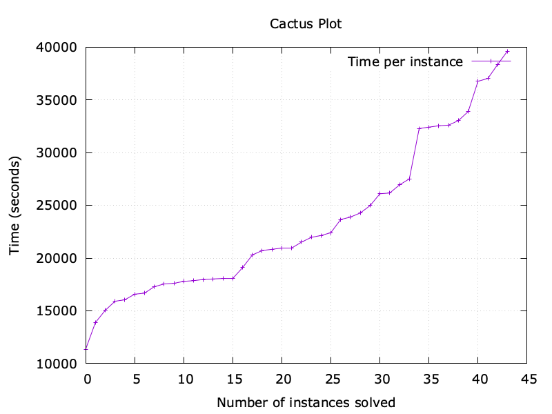
Full scale experiments. The plot below shows the time required to run the
bounded model checker for all executions of up to 6 transactions, to verify the
45 invariants in parallel. The plot shows the time in seconds that was required
to check each invariant, from the fastest one to the slowest one. As we can see,
the fastest experiment required about 3 hours, whereas the slowest experiment
required about 11 hours.
Degrees of confidence.
As can be seen from the short overview of the Quint techniques, random
simulation is the most straightforward and the fastest technique among the
three. However, it provides us with the lowest degree of confidence. For
instance, the probability of just choosing three specific transactions (e.g.,
SecurityCouncil::SoftFreeze, SecurityCouncil::HardFreeze, and
SecurityCouncil::Unfreeze) out of 20 available transaction types in that order
would be $\frac{1}{20^3} = \frac{1}{8000}$. If we multiply this probability by
the probability of choosing the right payloads, we will see that the chance of
producing a right sequence of transactions is quite low. The imprecision of this
technique is compensated by the speed of executing a single transaction
sequence. In our experiments, this technique has indeed missed multiple
invariant violations.
Randomized symbolic execution provides us with much better guarantees. As in the
case of random simulation, this technique may miss an invariant violation, when
it does not generate the right sequence of transaction types, e.g., the
probability of generating the sequence of three transactions is
$\frac{1}{8000}$, as we discussed above. However, once the right sequence has
been selected, the choice of right payloads is done by the constraint solver. As
a result, this technique has much better chances of hitting invariant
violations. In our experiments, this technique found multiple invariant
violations, but still missed a few. Since it runs the constraint solver in the
background, this technique is slower than random simulation, but it covers
significantly more executions.
Bounded model checking is the most complete technique among the three. If it
does not find an invariant violation for $k$ steps, it guarantees that there is
no sequence of up to $k$ transactions that draws values from the set of
predefined values and violates the invariant. In our experiments, this technique
found five invariant violations that were missed by the other two techniques.
However, it may take several days to analyze all executions, say, of up to 10
transactions.
7. Conclusions
It may seem non-obvious that we chose Quint for this task, instead of using
fuzzers or formal verification tools specifically designed for Solidity.
Interestingly, translating Solidity to Quint was not as much of a bottleneck in
this project, as one could have expected. Most of our time went into formulating
key invariants and understanding whether we had specified sufficiently many
invariants.
In general, we had a very fast feedback loop from writing an invariant to
finding a counterexample, if there was one. In addition to that, we used both
the randomized simulator of Quint, which is conceptually close to the fuzzer in
Foundry. After running the randomized simulator, to increase our confidence, we
were running the symbolic model checker Apalache, which is closer to symbolic
execution tools that are backed by SMT solvers. This required literally zero
boilerplate code, as the Quint tools are built on the concept of state
machines, invariants, and the temporal logic of TLA+.
]]>Igor Konnovigor@konnov.phdSpecification and model checking of BFT consensus by Matter Labs2024-07-29T00:00:00+00:002024-07-29T00:00:00+00:00https://protocols-made-fun.com/consensus/matterlabs/quint/specification/modelchecking/2024/07/29/chonkybftOr model checking fault-tolerant algorithms that have more states than the atoms in the universe
Author: Igor Konnov. Joint work with MatterLabs (Bruno França, Denis Firsov, Denis Kolegov, Grzegorz Prusak)
1. Introduction
Earlier this year, I was engaged by the Security Team at MatterLabs. They
needed help in formally specifying and checking the properties of the new
algorithm that was being designed by the Consensus Team. What intrigued me is
that the Consensus Team had the experience of implementing BFT algorithms with
their Era Consensus, but their new algorithm – called ChonkyBFT – existed
only in Rust-like pseudo-code. So the team wanted to start with a formal
specification before diving into a full-featured implementation. Since I had the
experience in specification and model checking of the
Tendermint consensus at Informal Systems, this seemed like a
feasible task to me.
This blog post summarizes the work done so far as well as the experience of
using pragmatic verification tools in a cutting-edge blockchain company. We have
checked a number of properties with Quint and Apalache. This is still a work in
progress, as we are constructing an inductive invariant, which would give us
even better safety guarantees than we have obtained so far.
If you want to skip the details and jump to the conclusions, here are the most
important outcomes of this work, in my opinion:
Our specification is type-correct and executable. Basic tests against the
specification are integrated into the CI on GitHub. Every time a change is
made to the protocol specification, a number of test scenarios are run in the
CI. You can play around with this specification instead of drawing
diagrams on a whiteboard.
We have conducted model checking experiments. These
experiments have uncovered relatively small inconsistencies in the informal
specification as well as a few missing message validation tests, which would
let the faulty replicas fork the system. Moreover, the model checker was
showing us breaking changes in a matter of several hours, whenever we
refactored the protocol. While several hours may sound like a lot, it is a
very fast feedback loop, compared to the manual protocol review.
In addition to that, we have adapted the Twins technique to Quint
specifications.
We have discussed the assumptions of the core consensus protocol about the
other protocols, for example, the interaction between the consensus protocol,
the block fetcher protocol, and the gossip layer. As a result, some parts of
the block fetcher were integrated into the core consensus protocol.
Due to the extremely large state space of the protocol, the model checker
was demonstrating significant slowdown in the analysis of some transitions. We
have identified a few problematic data structures. The Consensus team has
optimized these data structures without breaking the invariants. Not only has
this change visibly sped up the model checker, but it also decreased the size
of the messages.
To further mitigate the slowdown, we guided the model checker to detect
interesting examples faster, which can be done naturally in Quint.
In addition to confirming that the state invariants hold true, we have also
produced counterexamples to the invariants, when the number of faulty
replicas went over the expected threshold. This is a crucial step to
demonstrate that our specification is not over-constrained.
Interestingly, this work reinforces the vision of Quint, which I
presented at Gateway to Cosmos in 2023.
2. Choosing the specification language and tools
Before we started the specification efforts, we had to decide what specification
language to use. Obviously, I had plenty of experience with
TLA+ and Quint and all of the accompanying tools. Apart
from impressive expertise in protocol design, engineering, and testing, the team
at Matter Labs had previous experience with Alloy and Event-B.
Basically, we had two points of view, both of them valid:
The researchers knew from their previous experience that fresh verification
tools had a tendency to break in unexpected places. From that perspective,
when using Quint we had a risk of writing half of the formal specification and
then realizing that the tools were broken beyond repair. TLA+
tooling was much more mature and versatile.
The software engineers were saying that the Quint syntax looked much more
approachable than the syntax of TLA+. Moreover, Quint was offering
more familiar tools such as the randomized simulator and a testing framework.
As a result of this discussion, we arrived at the following compromise: We try
Quint, and if its tooling breaks beyond repair, I would rewrite the
specification in TLA+. Since the TLA+/Quint specifications
rarely go over 2 KLOC, and both languages build upon the same logic of
TLA+, it did not sound like a completely bizarre idea. In the end, we
did not have to rewrite our specification in TLA+, though I had to
work around several unimplemented features of Quint (more on this later). To our
luck, back at Informal Systems, we had built more solid tooling for Quint than
the typical minimal-viable-product approach required from us.
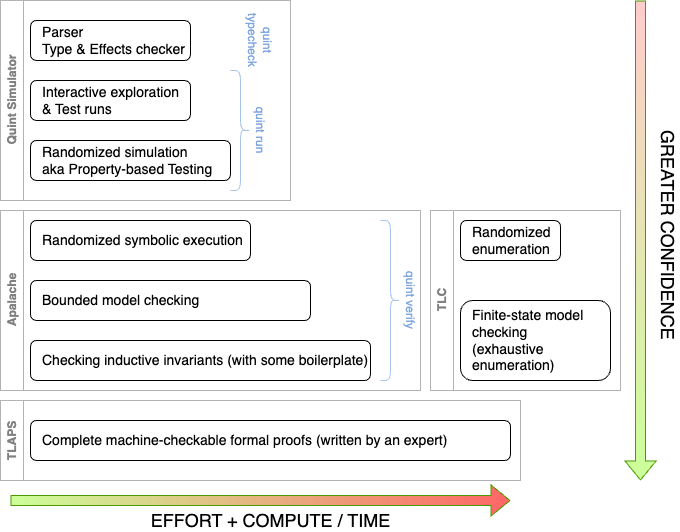
Figure 1. The spectrum of tools for Quint and TLA+
I will not go into details about the tooling offered by Quint and the
TLA+ infrastructure. It would be a good topic for a separate blog
post. Figure 1 captures the spectrum of the tools that are offered by
Quint and the TLA+ ecosystem:
Quint offers a testing framework similar to property-based testing. It
also has a randomized simulator that requires minimal expertise.
Apalache offers several approaches to symbolic execution and bounded
model checking via SMT solvers (satisfiability-modulo-theory solvers).
TLC implements exhaustive state enumeration as well as randomized
enumeration. (We have placed it to the right of Apalache in the figure, as TLC
would require immense resources to check the protocol that we are
investigating.)
TLAPS offers a proof system and a proof checker, also backed by SMT
solvers.
In this work, we have used a subset of the available tools: Quint’s tests and
its randomized simulator, Apalache’s randomized symbolic execution, and bounded
model checking. We are currently investigating whether we would be able to
leverage Apalache to show safety for unbounded executions by constructing
inductive invariants. Since we were doing model checking, we were able to
achieve greater degrees of confidence in the course of several weeks than we
would be able to achieve with naive testing or randomized simulation. However,
model checking is inherently incomplete in our setting, as it only proves or
disproves properties for fixed parameters. To achieve complete verification, we
would have to use a proof assistant such as TLAPS, Lean, or Coq,
which would require a much greater project budget than is typically allocated
for a security audit.
3. Distributed consensus in a nutshell
ChonkyBFT is a new Byzantine fault-tolerant protocol for distributed consensus.
It blends together recent inventions in distributed computing, e.g., quorum
certificates that can be traced back to HotStuff, the resilience condition
of $n > 5f$ like in FaB. The protocol also includes the own discoveries by
the Consensus Team.
In a nutshell, the BFT consensus works as follows. The distributed system is
composed of n replicas, up to f of which may be Byzantine: The faulty
replicas may simply crash, send messages to subsets of replicas, and send
conflicting messages to subsets of replicas. Importantly, the Byzantine
replicas can not forge the signatures of the $n - f$ correct replicas. To
keep things simple, we assume that $n > 5f$. In the more realistic setting, each
replica $n_i$ is assigned a weight $w_i$, and we assume that the sum of all
weights is at least five times greater than the sum of the weights of the $f$
faulty replicas. Under these assumptions, the minimal interesting network
configurations are as follows:
Six correct replicas: $n = 6, f = 0$. The algorithm should work correctly.
Five correct replicas and one faulty replica: $n = 6, f = 1$. The
algorithm should tolerate one faulty replica.
Four correct replicas and two faulty replicas: $n = 6, f = 2$. The
faulty replicas may break safety.
The goal of the replicas is to agree on the next block to commit onto a
blockchain. For specification purposes, the actual content of the blocks is
irrelevant. Hence, we assign some abstract values to blocks such as “val_0”,
“val_1”, or “inv_2”. As is common, most protocol operations are actually
done at the level of block hashes instead of complete blocks. The blocks are
involved only in a few cases, e.g., when a replica receives a proposal, or
when it receives a block from the gossip layer.
The correct replicas are progressing in views, starting with view 0. In every
view, a replica may receive a proposal from the view proposer
(programmatically known to all replicas), commit a block, issue a timeout, or
switch to the next view, as soon as it has received a justification to do so
(e.g., a timeout quorum certificate). When a replica receives a quorum of
commit messages for a certain block — signed commit votes from $n - f$
replicas — it commits a block. In this case, the replica also sends
the commit quorum certificate, so late replicas could catch up fast, instead
of aggregating quorums of their own.
The algorithm contains a number of optimizations for converging fast in the
“common case” when things go well, e.g., the network is responsive, and the
proposer for the current view is not faulty. In addition to that, the protocol
is optimized for the case of re-proposing the same block, when the replicas
have received sufficiently many commits from a sub-quorum of $n - 3f$
replicas. To this end, each replica stores the summary of the other
replica’s states that it has learned about by receiving messages, e.g., the
high vote, the high commit quorum certificate, etc. The concrete fields can be
seen in ReplicaState.
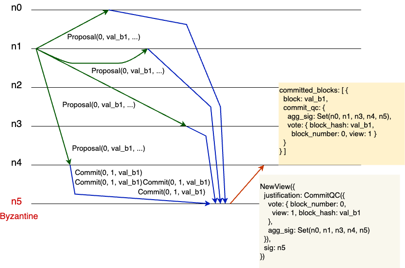
Figure 2. An example of replica 4 committing block “val_b1”
Figure 2 demonstrates a distributed computation of six replicas, with
replica n5 being faulty. Initially, replica n1 sends the proposal for the
block “val_b1” to be committed as the block number 0. The replicas $n_0$,
$n_1$, $n_2$, and $n_4$ receive this proposal and send their commit vote. The
faulty replica $n_5$ assembles the signed votes of $n_0$, $n_1$, $n_2$, and
$n_4$ and sends the new-view message that contains the signatures of $n_0$,
$n_1$, $n_2$, $n_4$, and $n_5$ itself. This is a perfectly valid message, as
$n_5$ could send a commit vote of its own. Finally, replica $n_4$ receives the
new-view messages, checks all the signatures, and commits the block “val_b1”,
since it has received a commit quorum certificate in the view message. This is
one of the shortest examples of just seven steps that were generated by the
model checker Apalache. The model checker produces output in Quint,
TLA+, and JSON. I drew the figure by hand, though one could automate
this process by parsing the JSON output.
If you want to see a concise description of the protocol, the best place to
start is with the informal specification in rust-like
pseudo-code. The description is actually quite concise, so the protocol may seem
to be deceivingly simple. Once you start asking questions about certain parts of
the protocol, it is probably a good time to switch to the formal
specification in Quint.
In terms of formal specification, we were mostly interested in showing the
safety of the protocol, that is, no disagreement on the blocks for the block
number, as well as in finding examples that would demonstrate its liveness, that
is, reaching a global state, where a correct replica commits one or more
blocks.
4. Choice of abstractions
Abstracting cryptography. The Consensus Team has chosen a good level of
abstraction when they were writing their informal specification. For instance,
the focus was on the distributed aspects of the protocol, assuming that the
cryptography primitives were working as expected. As real cryptography usually
stands in the way of automated reasoning, we immediately introduced common
abstractions: the hashes are perfect (actually, just the identity function), the
public and private keys are just node identities, etc. These definitions can be
found in types.qnt. For example:
// For specification purposes, a block is just an indivisible string.
// We can simply use names such as "v0", "v1", "v2". What matters here
// is that these names are unique.
type Block = str
// For specification purposes, we represent a hash of a string `s` as
// the string `s`. This representation is collision-free,
// and we interpret it as opaque.
type BlockHash = str
// Get the "hash" of a string
pure def hash(b: str): BlockHash = b
Tracking sent messages. Whereas an actual implementation of consensus would
have to send and receive messages by sending and receiving them over the wire,
our formal specification has the global view of the distributed system. Hence,
we simply store the sent messages and access them, whenever needed. For example:
// the set of all Timeout messages sent in the past
var msgs_signed_timeout: Set[SignedTimeoutVote]
// the set of all SignedCommitVote messages sent in the past
var msgs_signed_commit: Set[SignedCommitVote]
// the set of all NewView messages sent in the past
var msgs_new_view: Set[NewView]
// the set of all Proposal messages sent in the past
var msgs_proposal: Set[Proposal]
// ...
action on_proposal(id: ReplicaId, proposal: Proposal): bool = all {
  // [...]
  // Send the commit vote to all replicas (including ourselves).
  msgs_signed_commit' =
    msgs_signed_commit.union(Set({ vote: vote, sig: sig_of_id(id) })),
  // [...]
}
// ...
action replica_step_no_timeout(id: ReplicaId): bool = all {
  // ...
    all {
      msgs_signed_commit != Set(),
      nondet signed_vote = oneOf(msgs_signed_commit)
      on_commit(id, signed_vote),
    },
  // ...
}
Even though this approach to storing messages may seem to be too far off from
the actual implementation, this is actually a standard pattern of specifying
sent messages in fault-tolerant protocols. For instance, this pattern is used in
the TLA+ specifications of Paxos, Raft, and
Tendermint.
Faults. Since ChonkyBFT should tolerate Byzantine faults, we had to capture
the effects of Byzantine replicas in our specification. It’s often said that
Byzantine replicas may exhibit arbitrary behavior. Formal specification
languages force us to specify what “arbitrary” actually means. More precisely,
we have Authenticated Byzantine faults, which are defined by [Dwork, Lynch,
Stockmeyer’88] as follows:
Authenticated Byzantine: Arbitrary behavior, but messages can be signed with
the name of the sending processor in such a way that this signature cannot
be forged by any other processor.
We formalize a single step of the faulty replicas in the action called
faulty_step. Since its code contains about 160 LOC, we only show the
shortest piece that injects commit votes:
In the above code, an arbitrary subset of the Byzantine replicas inject their
commit votes for an arbitrary view, an arbitrary block hash, and an arbitrary
block number.
5. From tests to model checking and back to tests
In this section, I am going to be a bit technical. Keep reading though. The
main value of this section is not in the technical details, but in the
differences between the different approaches to experimenting with the
specification.
It is hard to write a complete formal specification from scratch, even if you
have an informal specification at the input. This is why I typically write
specifications incrementally:
Write the first specification of a simple state machine that captures only
a small but useful part of the distributed protocol. For example, the state
machine may only be able to send proposals, and there are no faults.
Run the Quint simulator via quint run and see whether the produced
examples make sense.
Add basic tests for the core definitions and run them via quint test.
Write a few more actions, e.g., receiving the proposals.
Add “falsy” invariants, that is, state invariants that are expected to be
broken. These invariants allow us to see that our specification is not
over-constrained. In other words, it is doing something useful. Check them
with the simulator via quint run.
When the tests become too hard to write, and the sample executions do not
help us to see anything new, it is time to write state invariants and check
them via quint verify, which, in turn, calls the Apalache model
checker.
At this point, many obvious invariants fail. This is why it is very
important to write as many of them as possible. It often happens that the
informal specification has trivial bugs, which would also be caught in the
implementation phase. It also happens that our state invariants are actually
wrong. This is the point when the model checker helps us a lot.
Enable faults in the specification and see how many state invariants become
broken again.
We basically followed the above methodology. Steps 1-5 look very similar to
normal software development practices and thus are often brushed off by experts
in formal methods. This is a grave mistake! These steps help the engineers to
build confidence in the formal specification. They stop seeing the formal
specification as an alien artifact and start seeing the value of having
specification code that just works at a different level of abstraction.
Writing tests. We wrote a small number of test scenarios. For instance,
replicas_normal_case_Test demonstrates a happy-path execution. In this test,
the correct replicas are committing three blocks. If you look at the code of
the test, you will notice that the test does not require any boilerplate, which
is common to see in the testing frameworks for distributed systems. The reason
is very simple: At this level of abstraction no boilerplate is needed! There are
no services to start and stop, no need to set up network interfaces, etc.
Actually, the test looks very much like an execution scenario that a researcher
or an engineer would write on a whiteboard.
What I like about Quint is that it naturally integrates the testing framework
and the interactive exploration. We can interactively repeat the steps of the
above test and inspect the intermediate states in REPL:
Checking falsy invariants. It is very easy to write a specification that
gets stuck somewhere in the middle. To avoid this, I usually write “falsy” state
invariants, which are meant to be violated. A violation would actually give us
an interesting execution that leads to the state we are looking for. For
example:
// check this invariant to see an example of reaching PhaseCommit
val phase_commit_example = {
  CORRECT.forall(id => replica_state.get(id).phase != PhaseCommit)
}
// check this invariant to see an example of having a timeout quorum:
val timeout_qc_example = {
  msgs_signed_timeout.map(m => (m.sig, m.vote.view))
    .size() < QUORUM_WEIGHT
}
Many of these invariants are simple enough so that the randomized simulator
finds counterexamples to them almost instantly:
$ quint run --invariant=phase_commit_example experiments/n6f1b1.qnt
...
The simulator helps us in finding basic executions that violate falsy
invariants. Once we are done writing simple falsy invariants, we write something
more exciting. For example, how about producing an execution, where at least one
replica commits a block:
// check this invariant to see an example of having a finalized block:
val one_block_example = CORRECT.forall(id => {
  not(replica_state.get(id).committed_blocks.length() > 0)
})
This looks like a nice invariant to get a counterexample to. Let’s try that:
$ quint run --max-samples=10000 --invariant=one_block_example experiments/n6f1b1.qnt
[...]
[ok] No violation found (584447ms).
Now what? Is our consensus protocol broken and it does not let us commit even a
single block? Luckily, we know that this is not true, as we have written the
test replicas_normal_case_Test earlier. Moreover, we have seen the example
in Figure 2. Phew.
We can throw more computing power. Since the Quint simulator is randomized, it
is trivial to run multiple instances of the simulator in parallel. All we need
is GNU parallel:
The above command runs 32 instances of quint run. We have to make sure that
these instances use different randomized seeds. Hence, we use the current date
concatenated with the instance number as a seed. Since we ask every instance to
execute 33k random runs, all instances simulate about 1 million runs together.
After running for two hours on a beefy machine, the simulator could not find an
execution, where one block was committed. Read further to see how it could be
faster with the model checker.
So far, we have been using more-or-less standard testing techniques that fit
under the umbrella of (stateful) property-based testing, e.g., see stateful PBT
in Hypothesis.
Model checking. Another way to quickly find a counterexample to
one_block_example is by running the Apalache model checker with quint
verify:
$ quint verify --invariant=one_block_example experiments/n6f1b1.qnt
[...]
[violation] Found an issue (1766648ms).
error: found a counterexample
It took the model checker about 30 minutes to find an example. Was it a bit
slow? Well, if we compare it with the randomized simulator, which could not even
find an example, it is not as slow.
Actually, we can find an example even faster, if we do not care about producing
the shortest example. To this end, we use randomized symbolic execution and
extend the maximal number of steps to 30:
$ quint verify --random-transitions=true --max-steps=30 \
  --invariant=one_block_example experiments/n6f1b1.qnt
[...]
[violation] Found an issue (229946ms).
error: found a counterexample
So far, we have been using the simulator and the model checker to find invariant
violations, when the invariants do not hold true. But what if the invariants do
hold true? We discuss this in the section below.
6. Making the specification slower
As we were progressing with the specification, we were adding more actions and
conditions to it. As a result, the model checking times were increasing. This is
not surprising, as Quint translates the specification to TLA+ and runs Apalache
under the hood. For such a rich specification such as the specification of
ChonkyBFT, Apalache generates hundreds of megabytes of SMT constraints, which
have to be discharged by the constraint solver called Z3.
At some point, we were not able to produce a counterexample to agreement for the
case of 4 correct replicas and 2 faulty replicas ($n=6,f=1,b=2$), even though
we knew that agreement should be violated in that case. Randomized symbolic
simulation was running for hours on 20 CPU cores, but every individual step of
it was so slow that we could not make much progress. We have found several ways
to fix this issue, see the following sections. Certainly, the best way was the
protocol optimization that was introduced by the Consensus team.
Under these circumstances, the easiest workaround is to get back to writing
tests. To make sure that the specification was still violating agreement in the
case of $n=6,f=1,b=2$, we wrote the test disagreement_Test. This test
demonstrated that, indeed, two faulty replicas could drive two honest replicas
into committing two different blocks for the same block number.
Of course, writing a test requires a very good understanding of the protocol and
some creativity. In particular, we had to find the right message payloads for
the test to work. Fortunately, this is where the model checker can help us in
saving the efforts, too.
7. Twins
Once our specification was way too complex for the model checker — we
fixed it later — we were looking into ways to analyze deeper properties
without waiting for days.
The first technique we looked at was the Twins technique, which was
originally applied to the consensus implementations. We are probably the first
ones who applied it to consensus specifications. Since it was shown to be
successful in testing actual implementations, we expected it to work well with
the Quint simulator as well. Without going into details about the twins, the
core idea is to let several replicas (the twins) run the correct code but give
them the same private key. Hence, the replicas that have the same private key
may vote differently in the same view, and this behavior will be perceived
externally as equivocation by a single replica, since the other replica would
not be able to distinguish between the twins.
It was relatively easy to introduce twins in our specification. In addition to
replica identities, we have also introduced a mapping from their identities to
the keys. For example, here is how we did it for $n = 6$ in twins_n6f1b1.qnt:
In the above specification instance, instead of having one honest replica
"n5", we had two honest replicas "n5_1" and "n5_2" that shared the same
key "n5". The key idea is that this behavior of two replicas "n5_1" and
"n5_2" is significantly simpler than Byzantine behavior in general. Our
expectation was that it would improve the performance of the Quint simulator,
since its execution space is much more constrained in comparison to the general
case.
It was easy to introduce the Twins technique. Unfortunately, it did not
help us in uncovering new behavior. For example, we could not find a
counterexample to agreement_inv for the case of four honest replicas and two
pairs of twins, which is specified in twins_n6f1b2.qnt.
8. Guided model checking
This section goes a bit into the guts of the Apalache model checker. If you find it too technical, just skip it.
Why does the model checker slow down? There are multiple reasons. The two most
obvious reasons are the following:
A large number of constraints are produced by the model checker, e.g., due
to a high degree of scheduling non-determinism.
The protocol has a large number of potentially reachable states.
We will see what we can do about the reason (2) in the next section. In this
section, we will see what could be done about (1).
What is a high degree of scheduling non-determinism? As is common in formal
modeling of distributed systems, an execution of a distributed system is
understood as a sequence of steps by individual replicas. In other words, we
consider all sequences of transitions made by replicas under all possible
interleavings (schedules). Since we specify potential transitions via actions,
we will talk about all possible interleavings of actions.
Let us have a look at the choices of transitions in the four steps of our
specification, starting from an initial state:
Step 1
Step 2
Step 3
Step 4
proposer_step
proposer_step
proposer_step
proposer_step
on_new_view
on_new_view
on_new_view
on_new_view
on_timer_is_finished
on_timer_is_finished
on_timer_is_finished
on_timer_is_finished
faulty_step
faulty_step
faulty_step
faulty_step
on_proposal_step
on_proposal_step
on_proposal_step
Let us have a closer look at the above table. In an initial state of the
protocol, we are in view 1. As expected, the view proposer may propose a block
by executing proposer_step. In addition to that, an honest replica may receive a
NewView message from view 0 — for a technical reason, the protocol is
bootstrapped by all honest replicas issuing timeouts in view 0. Also, an honest
replica may timeout. In addition to that, the faulty replicas can make a step.
All schedules. Now, I will tell you the secret about how the bounded model
checker in Apalache works. For the executions of up to 4 transitions, it
produces SMT constraints for all the actions in the above table. Then it adds an
assumption that only one of the actions may take place in every step. This adds
constraints for 19 potential steps. What is more important for understanding the
slowdown is that the solver has to consider all possible choices of the 19
actions in four steps. If you were solving systems of linear inequalities at
school, you can imagine how the solver would have to combine different cases.
Random schedules. Analyzing all executions at once seems to be wasteful.
What if we could analyze only one interleaving at a time? Without going into
definitions, this is what is usually called symbolic execution. Since in our
protocol many actions are enabled simultaneously, this would produce $4 \cdot 53
= 600$ interleavings and symbolic executions for just 4 steps! For this reason,
Apalache implements randomized symbolic execution. That is, an interleaving is
chosen at random, and a sequence of steps is encoded as symbolic constraints for
the given interleaving. By default, Apalache enumerates 100 such executions. In
practice, many interleavings are somewhat similar, they lead to the same states.
As a result, 100 random interleavings find bugs as good as enumerating 600
interleavings. If you are curious, there is a whole theory of eliminating
unnecessary interleavings, called partial-order reduction. Apalache does not
implement it though, falling back to randomization.
Guiding schedule selection. Now, enumerating all schedules is hard. Checking
them at random is easier, but there is a probability of missing an interesting
state. The model checker is completely unbiased towards any actions. For
example, it does prefer on_proposal_step over on_timer_is_finished. This is
also the power of the model checker, as it comes up with counter-intuitive
executions.
What if we do not want to start from an arbitrary initial state? Say, if we want
to find an example of two blocks being committed, we know that at least one of
them should be committed first. Hence, we could drive the protocol into a state,
where one block has been committed, and continue the search from there. This is
an example of guided model checking.
To our luck, we do not have to extend Apalache to get this behavior. The logic
of TLA+ behind Quint is so powerful that we can easily specify such a
scheduler in the language itself. To this end, we extend replica.qnt in
guided_replica.qnt. We have to introduce a bit of boilerplate code, due to the
current limitations of Quint, more on that later. The important declarations are
given below:
// the input trace to restrict the model checker's search space
const G_INPUT_TRACE: List[StepKind]
...
// remaining steps to replay
var to_replay: List[StepKind]
The trick is that we define a list of steps to replay. With every step, we
consume the head of to_replay and restrict the step, as prescribed by the head:
// initialize the replicas together with the trace to replay
action g_init: bool = all {
  init,
  to_replay' = G_INPUT_TRACE,
}

// execute the same actions as in replica::step,
// but restrict their choice with to_replay
action g_step = {
  any {
    // nothing to replay
    all {
      length(to_replay) == 0 or to_replay[0] == AnyStep,
      to_replay' = if (length(to_replay) == 0) to_replay else tail(to_replay),
      step,
    },
    // steps to replay
    all {
      length(to_replay) > 0,
      to_replay' = tail(to_replay),
      val expected_step = head(to_replay)
      any {
        all {
          expected_step == FaultyStep,
          faulty_step,
          unchanged_replica,
          leader' = leader,
        },
      ...
  }
Once we have done that, we can introduce a specialized version of the
specification that guides the scheduler according to G_INPUT_TRACE. Once the
schedule has been exhausted, the model checker starts its unrestricted
exploration, as in the general case.
For example, here is how we can initialize G_INPUT_TRACE to make all honest
replicas commit one block:
Importantly, we do not specify the gory details in this execution, e.g., which
messages are to be sent and received. Instead, we specify only the kinds of
steps and replica identities. In the case of OnNewViewStep, it’s also crucial to
submit the view. It’s the job of the constraint solver to fill in the gaps.
We used this approach to find an example of an honest replica committing two
blocks. It takes bounded model checker — verifying all interleavings
— a bit less than two hours to find an example of
two_chained_blocks_example:
$ quint verify --max-steps=50 --init=g_init --step=g_step \
  --invariant=g_two_chained_blocks_example n6f1b1_quided_one_block.qnt
...
[violation] Found an issue (5984680ms).
It takes just about five minutes to find an example with randomized symbolic
execution (since we are using randomization, the running times may significantly
vary):
$ quint verify --max-steps=30 --random-transitions=true \
  --init=g_init --step=g_step \
  --invariant=g_two_chained_blocks_example n6f1b1_quided_one_block.qnt
...
[violation] Found an issue (378368ms).
In our actual experiments, we were actually running randomized symbolic
execution in parallel on 16-32 CPU cores. This lets us produce examples even
faster.
9. Making the specification faster
At some point, we made an estimate of the potential state space. We considered
the following protocol configuration:
Six replicas, one of them faulty.
Up to 4 views.
Up to 2 valid blocks and 1 invalid block.
This configuration is probably the minimally interesting one. Yet, when we made the estimate of how many different messages could be sent by the Byzantine replica, the figure was really staggering:
$10^{410}$ messages!
When I started doing some preliminary work on finding an inductive invariant,
this figure became quite important. For inductive reasoning, we have to start in
a more or less arbitrary state. It became clear that one particular message type
could potentially carry plenty of data, especially if it was produced by a
Byzantine replica. This was due to the fact that a timeout quorum certificate
carried the votes of individual replicas, each of them being able to
additionally carry a commit quorum certificate.
During our meeting, the Consensus team immediately found a solution that would
dramatically reduce the size of timeout quorum certificates. As we have
specified this idea, model checking times were significantly reduced.
10. Model checking invariants that hold true
As we were writing the protocol specification in Quint, we were also formulating
state invariants. Such invariants were instrumental in catching typos and
missing validation tests in the protocol. One thing about auxiliary state
invariants that is rarely understood: Even though we could find some of the bugs
by checking safety properties such as agreement_inv, having a richer set of
state invariants helped us to detect the same bugs with the model checker much
faster.
The latest version of the protocol specification has 18 state invariants. Some
of them are relatively easy to understand. For example,
no_proposal_equivocation_inv checks that honest replicas do not cast different
proposals in the same view:
// a correct proposer should not equivocate for the same view
val no_proposal_equivocation_inv = tuples(msgs_proposal, msgs_proposal).forall(((m1, m2)) => or {
  not(m1.justification.view() == m2.justification.view() and m1.sig == m2.sig),
  FAULTY.exists(id => sig_of_id(id) == m1.sig),
  m1.block == m2.block,
})
Some invariants capture a deep understanding of the protocol. For example,
one_high_vote_in_timeout_qc_inv states that it should not be possible to
extract two high votes from a timeout quorum certificate.
We have also found these state invariants to be quite helpful in quickly
detecting issues that were introduced during protocol refactoring. For example,
the model checker produced an example that was exploiting a missing verification
of a commit quorum certificate. This issue was quickly fixed in the
Quint specification and the informal specification.
We have checked the invariants in several configurations:
Case $n = 6, f = 1, b = 0$: Six replicas, all of them honest.
Case $n = 6, f = 1, b = 1$: Six replicas, one of them Byzantine.
Case $n = 6, f = 1, b = 2$: Six replicas, two of them Byzantine. Many
invariants are violated in this case.
Case $n = 7, f = 1, b = 1$: Seven replicas, one of them Byzantine.
Since enumerating all interleavings takes too much time for ChonkyBFT, we
checked the invariants against 100 instances of symbolic execution of lengths up
to 25 steps. Since we ran the experiments multiple times, the actual number of
tried interleavings is well beyond 100.
11. The goodies and rough edges of Quint
On the positive, I find Quint tooling to be quite adequate for writing and
analyzing formal specifications of distributed systems. Obviously, I am biased,
since I have designed and developed large parts of Quint and Apalache. Here are
a few highlights of Quint tooling that I have found to be extremely useful in
this project:
Refactoring. Quint really shines at refactoring. Whenever the protocol
was changed, the type checker was reporting inconsistencies in multiple
places. While it was annoying to fix all these type errors one-by-one, it
would be much harder to spot them in an untyped specification language such as
TLA+.
Types. All mainstream programming languages use types. Hence, engineers
expect them, too. By defining types of the core data structures, we could
ignite the discussions about the protocol specification.
Tests. Unit tests and property-based tests are commonly used by
software engineers. In contrast to TLA+, Quint offers specification
writers a unit-testing framework. By leveraging non-determinism in Quint,
specification writers effortlessly extend unit tests to property-based tests.
Importantly, tests offer us a fallback option, when the model checker and the
randomized simulator are too slow.
Now that I have praised Quint, I should be honest and mention a few issues with
the tooling:
The module support still has issues. For instance, when we had to define an
instance for guided model checking in guided_replica.qnt, we had to
introduce boilerplate definitions to cope with the Quint parser.
The type errors reported by the type checker are not useful. It’s easier to
just ignore them and massage the types, instead of reading the messages.
Some recent language features break in unexpected places, e.g., I ran into
issues when using a user-defined version of the option type, see #1451.
Temporal operators are kind of supported, but there is not much
documentation.
In addition to that, we have felt lack of the following features:
It would be great, if the testing framework could verify the state
invariants in the intermediate states of the tests it is running. Since the
tests are already giving us non-trivial and important executions, we are
missing an opportunity there. We were manually adding such assertions in the
tests, but these assertions were distracting us from the core of the tests.
As we were discussing in the section on guided model checking, we extended
the specification to drive the protocol into states of interest. While the
model checker reaches those states faster in the guided specification, it
still takes some time to do it. It would be great, if the model checker could
save such intermediate contexts, and reuse them later.
If Quint supported some syntax for guided search, it would make our job
significantly easier.
In any case, there are no serious issues that could not be fixed by a dedicated
tooling team in six months.
12. Conclusions
I believe that we have brought great value to the project with our efforts in
formal specification and model checking with Quint and Apalache. We have already
summarized the benefits of using a specification language (Quint) and a model
checker (Apalache) in the introduction.
One issue with informal specifications is that they are open to interpretation.
Even if they look very much like code, different readers may understand various
pseudocode primitives differently. A specification language uses a fixed logic
interpretation that eliminates ambiguity. While a programming language also
fixes an interpretation – concurrency and non-determinism aside – specification
languages are much more concise than programming languages. This is especially
true for languages like Quint and TLA+, since execution efficiency is
not a concern. For instance, see my blogpost about memory in specifications.
In my experience, the real killer feature of our approach to specification is
the ability to quickly produce examples and counterexamples with the tools. This
helps all parties to get better confidence in the protocol. As there is no
single magic tool that is able to do that in all cases, we are using a portfolio
of tools and approaches: The randomized simulator, unit and property-based
tests, the bounded model checker, randomized symbolic execution, and guided
model checking.
As we have mentioned before, doing an exhaustive model checking of ChonkyBFT is
quite challenging, due to its rich behavior and the size of the potential state
space. Thus, we have mostly used randomized symbolic execution.While this
technique is surprisingly efficient at finding counterexamples, it is inherently
incomplete, that is, there is still a chance of violating some of the
invariants. Hence, we are investigating inductive reasoning for ChonkyBFT. Stay
tuned to read about our future results.
It is worth noting that analyzing consensus protocols is challenging in general,
and ChonkyBFT is no exception here. For example, see Formal Verification of
HotStuff by Leander Jehl (2021) and the PhD Thesis by Diego Ongaro on
Raft (2014), which both applied state enumeration with TLC. Byzantine faults add
another dimension to the problem, as Byzantine replicas produce incredibly large
state spaces. In this case, symbolic model checkers such as Apalache have a
better chance of succeeding, as exemplified by our earlier verification results
for Tendermint Accountability (2019-2020).
Do you want to receive notifications when I write something new? Subscribe to
the newsletter. New blog posts are going to be announced once per week (maybe
twice, if I really have something!).
]]>Igor Konnovigor@konnov.phdThe Rise of Model Checker: Verifying Blockchain Monitors In and Near Realtime (Solarkraft #5)2024-07-19T00:00:00+00:002024-07-19T00:00:00+00:00https://protocols-made-fun.com/solarkraft/2024/07/19/solarkraft-part5
In this post we first formally define what hybrid blockchain runtime monitors are (from the formal methods point of view), as then proceed to explore the far-reaching avenues of how to go from offline monitoring, as done now in Solarkraft, to truly online monitoring on the live blockchain.
Verifying Runtime Monitors on a Blockchain 📒
After reading the previous post on hybrid blockchain monitors you may say: “All that is nice and good, but here are a few questions that still need to be addressed…” For people with different backgrounds these are probably the main ones:
🕴CEO / CTO: “Huh? Formal methods? Why do I need yet another monitoring solution? I already have the X/Y/Z system, and they send me real-time alerts!”
🤓 Formal methods person: “How do you verify blockchain monitor? What are your verification conditions?”
👨🏫 Mathematician: “What about verification complexity?”
🧔 Software engineer: “How do you practically check them on the live blockchain?”
This blog post outlines the answers to the above questions. TL;DR:
Formal methods-based blockchain monitors offer a unique combination of conciseness and completeness: formal monitor specifications are extremely compact, but, at the same time, they allow to completely specify and differentiate valid/invalid transactions, and to detect and prevent a wide range of potential errors or exploits, which are out of reach of traditional alert-based monitoring solutions.
We verify blockchain monitors via a) producing verification conditions from each monitor specification; b) extracting pre- and post-states for every relevant blockchain transaction, as well as its parameters; c) validating each transaction against verification conditions using the Apalache model checker.
Complexity of verifying blockchain monitors is linear wrt. the number of conditions in the specification and the number of transactions: each condition is checked at most once against every transaction (but many checks may be skipped/optimized away). On the other hand, the inherent logical complexity of checking individual verification conditions is highly dependent on their nature, and may be both very low and very high; it depends. We do propose below some ways to combat this complexity, exploiting for that the modular nature of our monitors.
Practically, in the current Solarkraft system, we verify blockchain monitors in offline mode by first downloading transactions using solarkraft fetch, and then verifying them using solarkraft verify; as this doesn’t allow to execute preventive measures, we want to move eventually into verifying monitor specifications on the live blockchain, i.e. we want to do online monitoring. There may be several intermediate-strength solutions to that problem, which we outline below.
Caught your attention? Do you want a monitoring solution for your blockchain project? Give us a ping! We are always happy to talk to you:)
Are you interested in more details? Then continue reading!
Formal Blockchain Monitors are Super-Powerful 🦸
In this section we answer the question from an imaginary CEO/CTO:
“Huh? Formal methods? Why do I need yet another monitoring solution? I already have the X/Y/Z system, and they send me real-time alerts!”
As a general intro into the usefulness of runtime monitoring for blockchains we recommend the first episode from our blockchain series: “A New Hope – Why Smart Contract Bugs Matter and How Runtime Monitoring Saves the Day”. But from the question we conclude that our CEO is already convinced that monitoring is useful, and is even using some other monitoring solution. So, why do we need formal methods-based blockchain monitors?
To answer that question, let’s see what a typical blockchain monitoring solution offers:
receive real-time alerts and notifications about blockchain events
understand usage patterns and fund flows with customized dashboards
understand the risk of a transaction; simulate its outputs in real time.
Typically, some or all of the above activities can be parameterized, e.g. wrt. the addresses, or kinds of transactions, or amounts of funds, etc., which gives these systems a certain level of flexibility. Still, a typical monitoring system suffers from two main drawbacks:
Prevention techniques offered by typical monitoring systems are most often incomplete: it is impossible to describe by any fixed set of rules the correctness conditions for an arbitrary smart contract.
When attempts are made within standard monitoring systems to improve their completeness, these attempts usually lead to proliferation of more and more complex pattern-based rules, which are cumbersome to create and maintain, while still never achieving the necessary completeness level.
“Real-time alerts” happen post-factum, when the transaction has already committed its changes. This is already too late: receiving a notification that funds have been withdrawn doesn’t help returning them.
Some systems try to prevent harmful events by using throttling, i.e. limiting the amounts of fund transfers within a period of time. While helping to mitigate the harmful effects to some degree, these solutions are also unsatisfactory for two reasons: a) they can still be side-stepped (e.g. by decreasing the withdrawal speed, or using intermediaries); b) throttling restrictions lead to frustrating experience for legitimate users.
Notice that the first problem (monitoring incompleteness) is exactly the reason for the second problem (post-factum response, lack of harm prevention): without being sure that we have described all possible valid/invalid cases, we can’t really be sure to revert a transaction, even if we suspect it being harmful.
Here is where formal methods-based blockchain monitoring comes to save the day. Formal methods offer a mathematical logic-based solution which allows in many cases to completely specify and differentiate valid/invalid transactions. Moreover, using such decades-proven specification languages as TLA+ helps to do it very compactly, and employing such powerful symbolic model checkers as Apalache allows us to check formal specifications extremely fast, in fractions of a second.
We want to seamlessly integrate complete validation of transactions against monitor specifications directly into the transaction execution lifecycle. With our current Solarkraft system we have made the first step towards this ultimate goal of online blockchain monitoring; in the subsequent sections we elaborate in more details about the technical details, as well as the next steps towards our goal.
Blockchain Monitors in Formal Attire 👔
In this section we define, using mathematical notation, what blockchain monitors are, and how to verify whether a blockchain transaction satisfies the conditions expressed by a monitor.
Formally, a blockchain is a sequence of ledgers, where each ledger is a snapshot of the blockchain environment and the blockchain state. States are partitioned: first into separate spaces per contract, and then into separate regions per contract variable. Blockchain states are mutated by transactions, where each transaction is an invocation of a certain contract method with the corresponding method parameters supplied. The invoked method modifies the states according to its logic. A successful transaction bring the blockchain from one environment/state to the next; a rejected/reverted transaction leaves the blockchain environment/state unchanged. We assume that unsuccessful transactions can be still observed.
We employ the following notation:
\(D\) is the set of all possible data values: strings, numbers, structs, etc. Mathematically we don’t distinguish between different data types (though practically we of course do).
\(V\) is the set of typed contract variables. At this stage we don’t distinguish between states of different contracts: logical assertions may refer to the state of any contract (e.g. to token balances in other contracts).
\(S = S_0, S_1, ...\) is a sequence of states.
\(S_i \subseteq V \mapsto D\) is the \(i\)-th contract state, which is a partial mapping from variables to their data values. If a variable \(v\) is present in the mapping \(S_i\), we say that it is defined in this state.
\(T = T_0, T_1, ...\) is a sequence of transactions. Each transaction brings the contract into its next state, which we denote by \(S_i \xrightarrow{T_i} S_{i+1}\).
\(P_T\) is the set of all possible typed method parameters.
\(T_i \subseteq P_T \mapsto D\): each transaction is a method invocation, represented by a partial mapping from method parameter names to their values; only the parameters specific to the invoked method are present in the mapping.
\(E = E_0, E_1, ...\) is the blockchain environment, which is a sequence of environment states; each transaction executes in a specific environment state.
\(P_E\) is the set of all typed environment parameters (such as current_contract_address, ledger_timestamp, or method_name).
\(E_i: P_E \mapsto D\) is a mapping from environment parameters to their values, and defines the current blockchain environment, in which \(T_i\) executes.
\(X_i \in \mathbb{B} = \{ \top, \bot \}\) is the result of executing the transaction \(T_i\): \(\top\) in case of success, \(\bot\) in case of failure.
The above definitions describe the structure of the object to which we apply monitor specifications: a smart contract, executing on a blockchain. Now it’s time to define the structure of monitor specifications themselves. As checking each direct method specification or reverse effect specification is independent from others, we define only the structure for individual monitors.
\(M_D = \langle F, P, H \rangle\) is a direct method monitor specification, where the components are the finite sets of MustFail, MustPass, and MustHold conditions respectively.
\(M_R = \langle C, A \rangle\) is a reverse effect monitor specification, where the components are the finite sets of MonitorCheck and MonitorAssert conditions respectively.
In the above:
For any \(F_j \in F\), \(P_k \in P\) we have \(F_j, P_k: (E_i, S_i, T_i) \mapsto \mathbb{B}\) are boolean conditions of the environment state, the past contract state, and the method parameters.
For any \(H_j \in H\) we have \(H_j: (E_i, S_i, T_i) \times S_{i+1} \mapsto \mathbb{B}\) are boolean conditions of the environment state, the past contract state, the method parameters, and the next contract state.
For any \(C_j \in C\), \(A_k \in A\) we have \(C_j, A_k: (E_i, S_i) \times S_{i+1} \mapsto \mathbb{B}\) are boolean conditions defined over the environment state, the past contract state, and the next contract state.
Verification Conditions for Blockchain Monitors
Verification conditions are verifiable mathematical statements, which encode a certain aspect of the system correctness; in our case they encode whether the blockchain transaction is correct wrt. the blockchain monitor. Having formally defined what are blockchain states, transactions, and monitors, we are now in a position to specify monitor verification conditions.
For a direct blockchain monitor \(M_D = \langle F, P, H \rangle\), we combine individual monitor conditions into larger ones:
Compare these formal verification conditions with the informal conditions from the previous post, as well as with the TLA+ encoding of verification conditions for Timelock’s deposit method. Notice also that the two implications from the pairs “Must fail”/”Failure completeness” and “Must succeed”/”Success completeness” encode together an equivalence between the checks and the transaction execution result. Nevertheless, we consider it a better strategy to treat these conditions separately, as this allows the developers to encode a more fine-grained monitor response. For example, a monitor may forcefully revert a transaction that violates the “Must fail” condition, but only issue a warning when “Failure completeness” is violated.
For a reverse blockchain monitor \(M_R = \langle C, A \rangle\), we also combine individual monitor conditions into larger ones:
Model checking is an automatic procedure of verifying mathematical specifications. Within Solarkraft, we employ TLA+ as our specification language, and Apalache as our model checker. Here are a few details worth noting:
Apalache is a general purpose model checker, in that it performs invariant checking: given an initial system state \(\mathit{Init}\), an encoding of the system transitions (the next-state relation) \(\mathit{Next}\), and an encoding of a supposed system invariant \(\mathit{Inv}\), it checks whether the invariant does indeed hold in all system states reachable from the initial one by executing system transitions.
Apalache is a bounded model checker: it can check invariants only in states reachable in a certain number of transition steps (the execution bound \(\mathit{Length}\), say 1, 5, or 10) from the initial state.
Apalache is a symbolic model checker, i.e. it encodes the the verification conditions symbolically, as formulas in certain logical theories, and passes the resulting encoding to Satisfiability Modulo Theories (SMT) solvers, which are specialized tools for solving massive volumes of math equations.
In the current system we employ Apalache by encoding monitor verification conditions as a deadlock checking problem: we encode the verification condition as part of the next-state relation. Thus, if the verification condition is violated, the system is unable to proceed (there is a deadlock), and this is detected by Apalache. Formally, for any given blockchain environment \(E_i\), the transaction pre-state \(S_i\), the transaction being executed \(T_i\), the transaction execution result \(X_i\), the transaction post-state \(S_{i+1}\), as well as any of the above verification conditions \(\mathit{VC}\), we execute Apalache using the following encoding:
A few TLA+ tests for Apalache verification conditions using this encoding can be found e.g. in deposit_test.tla (for the direct monitor of Timelock’s deposit method), or in balance_record_test.tla (for the reverse balance record monitor). In all cases Apalache is invoked in a similar fashion, e.g. like that for deposit’s first test:
As explained above, Apalache is a bounded model checker: it can check execution traces up to a certain bound on the execution length. For most systems this restriction starts to manifest itself from the execution depth of around 7 steps: the model checker slows down substantially when exploring execution traces longer than that. But specifically for monitoring this restriction is irrelevant: with the execution length of 1 Apalache is blazing fast, and verifies the above formulas in fractions of a second, so it’s a perfect choice for monitoring applications.
In the above tests a monolithic encoding is used: all monitor conditions are encoded as a single invariant, and also included into the next-state relation. This encoding is the compromise we had to make due to the very limited project timeline, and has a few drawbacks:
All verification conditions are lumped together into a single invariant, and, moreover, the invariant is part of the next-state relation. As a result, when the invariant is violated, the feedback from the model checker is suboptimal: it reports only that the system is unable to proceed (deadlocked), but doesn’t explain the reason for that (as no invariant was violated).
In cases more complex than Timelock, verifying a single large invariant may become way more time-consuming than the sum of times for verifying each individual invariant separately, due to ultimately exponential nature of the resulting logical problem.
In general, we can be more flexible in encoding monitor verification conditions for model checking. E.g. in another version of Timelock’s monitors we encoded one combined monitor condition per invariant. Finally, verification conditions can also be encoded very fine-grained, down to the smallest scale, when an invariant to be checked contains a single direct monitor condition (one of \(F_j\), \(P_j\), \(H_j\)), or a single reverse monitor condition (one of \(C_j\), \(A_j\)). In all those cases, we encode a verification condition \(\mathit{VC}\) as an invariant checking problem for Apalache in the following way:
This encoding solves the aforementioned problems wrt. monolithic encoding: the feedback from the model checker explains in details what is the problem when an invariant is violated; the encoding can also provide substantial improvements in terms of execution speed for monitors which are more complex than Timelock’s.
Practical Checking of Blockchain Monitors 🛠
In the present Solarkraft system we do what’s called offline monitoring: we verify monitors after the state has already been committed to the blockchain. The delay between the action and the response can be made very small, a few seconds, but due to the final nature of the committed transactions this is not enough: the changes (such as balance transfer) can’t be undone. Our eventual goal is to perform online monitoring, i.e. to verify the monitors before the state has been committed, in order to be able to do preventive actions. This far-reaching goal is non-trivial, and has a few intermediate-strength solutions, which we are about to explore now.
Offline monitoring is is the simplest blockchain monitoring solution, applied both by standard blockchain monitors, as well as by our current Solarkraft system:
A transaction is committed on the blockchain;
At some later time point, the transaction effects are observed: solarkraft fetch;
Transaction is validated, and acted upon: solarkraft verify --alert.
This approach is useful in that the reaction to the event (a transaction) may happen in near real time: a few seconds later. The problem is that for blockchain this is not enough: what matters is the logical state on the blockchain, which, when committed, is irreversible (except for hard forks). Thus, in many cases, the reaction can’t prevent the possible harm being done.
To better understand how preventive actions may be done, let’s take a look at Stellar’s transaction lifecycle. The important points where a monitoring system may intervene in the transaction lifecycle are the steps 3, 7, and 10:
Creation (Transaction Creator)
Signing (Transaction Signers)
Submitting (Transaction Submitter): After signing, the transaction can now be submitted to the Stellar network. If the transaction is invalid, it will be rejected immediately by Stellar Core.
Propagating (Validator)
Crafting a candidate transaction set (Validator)
Nominating a transaction set (Validator)
Stellar Consensus Protocol (SCP) determines the final transaction set (Validator Network). SCP resolves any differences between candidate transaction sets and ultimately determines a single transaction set to apply, the close time of the ledger, and any upgrades to the protocol that need to be applied network-wide at the apply time.
Transaction apply order is determined (Validator Network)
Fees are collected (Validator)
Application (Validator): Each transaction is applied in the previously-determined order. For each transaction, the account’s sequence number is consumed (increased by 1), the transaction’s validity is rechecked, and each operation is applied in the order they occur in the transaction. Operations may fail at this stage due to errors that can occur outside of the transaction and operation validity checks. For example, an insufficient balance for a payment is not checked at submission and would fail at this time.
Protocol Upgrades (Validator)
Why are these steps important? Because exactly at these steps new information appears, which influences transaction validity:
Step 3: the transaction \(T_i\) is determined: its parameters, signatures, etc.
Step 7: the blockchain environment \(E_i\) is determined, in which \(T_i\) will execute:
the set of transactions which will be executed together with \(T_i\);
\(T_i\)’s ledger number / timestamp;
the starting state for ledger’s transaction set, which is the end state of the previous ledger.
Step 10: the starting state \(S_i\) for transaction \(T_i\) is determined, which is the result of applying all other transactions preceding \(T_i\) in the apply order determined at step 8.
It is worth noting that the order of application determined at step 8 is also a new piece of information, which influences transaction validity (and ultimately determines \(S_i\)). Nevertheless, as steps 8-10 happen essentially at the same time (see LedgerManagerImpl::closeLedger), this difference in timing is immaterial. For conceptual reasons we prefer to focus on step 10.
When speaking about practicality, timing and throughput parameters start playing an important role:
Typical Stellar ledger close time: 5-6 seconds
Stellar transaction throughput (transactions per second, TPS): up to 1000
What does the above mean for validating blockchain monitors? Two things:
With each step, additional data becomes available; thus more monitor verification conditions (VCs) can be validated:
At step 3: stateless VCs can be validated, i.e. those depending only on \(T_i\);
At step 7: semi-stateful VCs, depending only on \(T_i\) and \(E_i\) can be validated;
At step 10: all stateful VCs can be validated.
With each step, the timing constraints become more strict (in order not to disrupt the core blockchain functionality):
At step 3: any reasonable time (e.g. up to 10 seconds) can be allocated to execute the transaction validity checks;
At step 7: a small portion of the ledger close time (e.g. up to 1 second) can be allocated for checking all ledger’s transactions;
At step 10: a tiny portion of ledger close time (e.g. up to 100 milliseconds) can be allocated for checking all ledger’s transactions.
What can Apalache model checker checker offer us in terms of validity checks execution time? For the Timelock example, the typical VC check time is around 1 second on a powerful laptop. Using such features as Server Mode (mostly implemented, see [FEATURE] Server Mode and RFC-010: Implementation of Transition Exploration Server) we expect the startup time (runtime setup, parsing, typechecking, preprocessing) to be amortized for multiple queries, and validity checking time to be reduced to something like 100 milliseconds. This sounds good! But a few problems still exist, unfortunately:
This is the checking time for a single transaction; but for steps 7 and 10 all ledger’s transactions need to be checked. Taking into account the blockchain parameters, this means checking up to 5000 transactions in 1 second (for step 7), or in 100 milliseconds (for step 10).
The Timelock example is one of the simplest imaginable in terms of its logical complexity. Thus, for more complex examples the checking time can be substantially higher.
Taking all of the above in consideration we have two (mostly independent) strategies of how blockchain monitors can be integrated into the transaction lifecycle: one from formal methods point of view, and another from blockchain engineering point of view.
Model Checking Improvements for Blockchain Monitoring
As can be seen from the analysis above, model checking has to provide hard real time execution guarantees for validity checks,
such as “up to 5000 transactions can be checked in 100 milliseconds”. How can this be done? Below are a few ideas on how to achieve that.
Software engineering improvements. Features such as Server Mode can substantially reduce startup times, giving up to 10x checking time reduction. This feature is mostly implemented, but still needs some polishing. Another useful feature would be efficient parallelization (also partially implemented): given 5000 transactions, each independently checkable in 100 ms, and being able to execute the checks in parallel, would allow us to execute all ledger’s transactions checks in 100 ms.
Model checking problem decomposition. Our hybrid blockchain monitors are already quite modular, in the sense that each monitor is expressed as a combination of simple conditions. As we explained in the previous sections, the verification conditions can be checked independently for each monitor condition, and then combined at the boolean level. Solving each of the resulting subproblem independently will allow both for parallelization (see above), as well as to use specialized solvers for each subproblem, with different complexity constraints (see below). We could employ the three-valued logic to describe the boolean structure of the overall problem, with the Unknown value expressing that the model checking is not possible with the available information, or didn’t terminate within the required hard time bound. Using then logical connectors from the three-valued logic would allow us to provide meaningful answers in some cases when the standard model checking procedure would not terminate.
Theory-specific solvers for subproblems. Apalache reduces model checking problem to the QF_NIA logic (Quantifier-free theory of nonlinear integer arithmetic). While being very general and powerful, this theory is in the worst case undecidable. When looking at moderately large model checking problems as a whole (even at Timelock) at least QF_LIA (Quantifier-free theory of linear integer arithmetic) is required, which is a subtheory of QF_NIA with exponential complexity. When looking at subproblems though, simpler theories could be employed; examples of those are QF_EUF (Quantifier-free theory of equality and uninterpreted functions) with the worst-case \(n \cdot \mathit{log}(n)\) complexity, or QF_IDL (Quantifier-free theory of integer difference logic), with the worst-case cubic complexity. Putting aside record access (which can be abstracted away in some cases) examples of subproblems with reduced complexity in the Timelock case can be found in the Balance Record monitor, which falls under QF_EUF theory, or Claim’s MustHold monitor conditions, which is expressible in QF_IDL theory.
Blockchain Engineering for Runtime Monitoring
All of the above model checking improvements are useless if they can’t be applied at the right time and place. For that, a proper integration of monitoring into transaction lifecycle is necessary, specifically to be able to execute preventive measures when a violating transaction is detected. Based of the transaction lifecycle outlined above, here is how we see this can be done:
Execute stateless validity checks at transaction submission time. At step 3, when a transaction is submitted to the blockchain, stateless checks (depending only in \(T_i\)) can be executed; this needs to be done at Stellar Core, as the single controllable point of entry for all incoming transactions. As timing requirements are not too strict at that point, Apalache can be employed as is (only the software engineering improvements would be useful for efficiency reasons).
Execute semi-stateful validity checks when SCP decides ledger’s transaction set. Semi-stateful checks (depending on \(T_i\) and \(E_i\)) can be executed at step 7 by the validator network; the timing requirements become moderately strict, so model checking problem decomposition becomes necessary.
Execute stateful checks when transactions are applied. This is done by a validator node at step 10, and the timing requirements are the most strict ones, so all model checking improvements become necessary. Inevitably there will be cases when model checking will exceed the timing requirements, returning the Unknown answer, so the monitoring system should be configurable with actions to be executed when this happens. E.g. in the most critical cases a transaction can be reverted; in less critical cases a transaction may be allowed to pass, but an alert will be issued.
All of the above requires integration of formal-methods based monitoring into the central blockchain components. If this isn’t possible for some reason for the whole blockchain, what can a project do in order to implement individual project monitoring? Though it’s less efficient than the whole-blockchain solution, but a lot can still be done:
Perform stateless validation of user transactions via a dedicated service. A project may require its users to submit transactions using Permits via a centralized service, which will perform transaction validation by interacting with the monitoring system. The service, in case of successful checks, will sign and submit transaction to the blockchain. The on-chain components of the system need to be restricted to accept only such transactions which are signed by the service, and also validate user’s Permit signatures.
During transaction processing, perform stateful checks via on-chain monitoring system. An on-chain monitoring system can be implemented which will perform (limited) transaction validation. A project-specific contract, when receiving a transaction, will call into the monitoring system to perform transaction validation. This in turn can be done in two ways:
Implement on-chain solvers for simple theories such as as QF_EUF or QF_IDL, and validate the transaction within the same call. Some attempts in that direction have been undertaken already for EVM/Solidity, see e.g. the pilot project EVM Symbolic Execution in Solidity.
Accept transaction for validation, log it on-chain, and wait for an off-chain component to validate it. The off-chain component will commit the validation results on-chain, and the on-chain component will forward the result to the project-specific contract. This happens with an inevitable delay of at least 1 ledger: e.g. a transaction is submitted at ledger \(n\), but validated and executed at ledger \(n+1\). While slightly less convenient for the user, this allows to side-step hard real time requirements wrt. model checker execution.
This post concludes our blog post series about the first phase of Solarkraft development; we hope you’ve enjoyed it. Please don’t hesitate to write to us: we are happy to hear from you, and discuss everything concerning the fascinating topic of blockchain runtime monitoring!
While the previous posts explain the current state of the project, in this one we take one step further, and explore the directions in which we plan to evolve blockchain runtime monitoring with Solarkraft. Throughout the post we are using the same timelock contract from soroban-examples that was used in Part 2: “Guardians of the Blockchain”; please explore at least this post first to acquire the necessary context.
Blockchain Runtime Monitors
Runtime monitoring, also known as runtime verification, is a well-established field, where many practical approaches have been devised and applied successfully. Based on this heritage, we proposed the first version of a Web3 runtime monitoring system for the Stellar blockchain in Part 2: “Guardians of the Blockchain”. Our system is based on the TLA+ specification language, a well-established formalism for specifying and verifying distributed systems.
Taking a step back from the concrete solution, let’s try to answer the more abstract question: What do we want to achieve with runtime monitors in blockchains? As runtime monitors are eventually going to be deployed and executed on the live blockchain, they should satisfy the following requirements:
Prevent from safety violations (safety): bad things, such as your token balance being stolen, should not happen. This is the primary goal of runtime monitors: react preventively, and abort unwanted executions.
Detect liveness violations (liveness): good things should be able to happen! E.g. you, as an account owner, should be able to withdraw your own balance. If a legitimate transaction keeps reverting, that’s also a bug, not less severe than someone stealing your tokens.
Detect unexpected behaviors (completeness): same as code, specs are not perfect. If a spec author overlooked some behaviors, and they manifest themselves on the live blockchain, this may mean anything: from simple spec incompleteness, to an exploit being executed. Monitors should be configurable to either issue a simple warning, or to prevent such behaviors altogether.
The problem we’ve observed with the previously employed approaches to formal specification is that the specs of what the method should do can easily be much larger than the actual implementation. So we would like to add to the above the following soft requirement:
Specify behaviors compactly and independently (compactness and modularity): it is usually the case that a smart contract encompasses a lot of various aspects (e.g. authentication, authorization, storage management, math computations), and is written/employed/reasoned about by various roles (e.g. smart contract developer, mathematician, architect, UI developer). All of those roles should be able to specify various aspects of the smart contract behavior as easily and as independently as possible.
So monitors should be able to specify both safety and liveness properties, be complete wrt. the current and future system behaviors, and, preferably, also be compact and modular. For that we propose a conceptual separation of monitors into direct monitors (those reasoning from cause to effect), and reverse monitors (those going from effect to cause). We can combine the two together in what we call hybrid monitors.
Direct Monitors
Here we reason from the cause (method invocation) to the effect, but apply a structure which closely mimics, in formal semantics, what we expect to see when we program smart contracts. The essence of the structure is in the picture below:
In direct monitors, we distinguish three kinds of conditions:
MustFail_i is a condition under which the method is expected to fail. If any of those conditions hold, the monitor activates, and checks that the method does indeed fail;
MustPass_i is a condition, under which the method is expected to succeed, provided that none of the MustFail_i conditions hold. Each MustPass_i condition represents a separate happy path in the method invocation;
MustHold_i is a condition that should hold after the method invocation is successful (e.g. the tokens should be transferred). Unlike the previous two categories, which reason only about the state of the system before the method invocation, these properties may reference both the post-method state, and the pre-method state. All of MustHold_i should hold if the method is executed successfully.
In the above, Must<Fail|Pass|Hold> is a prefix, which tells the monitor system how to interpret this predicate. The complete pattern for predicate names with these prefixes is as follows:
All predicates which refer to the same <Method> will be grouped, to create together one method monitor. Interpreted formally, the monitor should do the following when <Method> is invoked:
If any of MustFail_i conditions hold, check that method invocation reverts (otherwise, issue a warning / revert if configured to do so)
If none of MustFail_i conditions hold, but method invocation reverted, issue a warning (incomplete spec)
If none of MustFail_i hold, and one of MustPass_i conditions hold, check that method invocation succeeds (otherwise, issue a warning)
If none of MustFail_i hold, and none of MustPass_i conditions hold, but method invocation succeeded, issue a warning of an incomplete spec (or revert if configured to do so)
If method invocation succeeds, check that all of MustHold_i conditions hold on the pre- and post-states of the method invocation (otherwise, issue a warning / revert if configured to do so)
Notice that above we apply or as default connector for preconditions (MustFail_i / MustPass_i), and we apply and as default connector for effects (MustHold_i). Thus, you may split preconditions/effects into separate predicates at your convenience, avoiding complicated logical structure inside predicates themselves.
Direct monitors for the Timelock contract
Having outlined the general structure of direct monitors, let’s apply it to the Timelock contract. Direct monitors for Timelock’s deposit and claim methods can be found in deposit.tla and claim.tla respectively; below we depict only the structure of these monitor specifications (we omit Must<Fail|Pass|Hold> as well as the method names for clarity).
As can be seen, a direct method monitor is decomposed into a collection of independent and small monitors, i.e. we did achieve our (soft) goal of compactness and modularity. Safety and liveness goals also seem to be satisfied:
Safety: Timelock’s direct monitors guarantee numerous safety properties. A safety property is usually ensured by either MustFail, or MustHold, or a combination of both conditions. For example:
The property “only the approved claimant may claim the deposit” is ensured by the NonClaimant sub-monitor;
The property “the Timelock contract receives the deposited funds from the claimant” is ensured by the combination of NotEnoughBalance and TokenTransferred sub-monitors.
Liveness: Timelock’s liveness properties are guaranteed by the MustPass conditions:
Implicit in case of deposit (whatever doesn’t fail, should succeed);
Explicit in case of claim: a claim happening before the time bound, when its kind is Before, should succeed due to BeforeTimeBound (provided all other conditions are met); similarly, a claim happening after the time bound, when its kind is After, should succeed due to AfterTimeBound.
Can the described approach of direct monitors be considered satisfactory? Please stop to think about it for a sec, before opening our answer below.
Are direct monitors sufficient?
You may have guessed the answer: we believe NO! And here is an (incomplete) list of reasons why:
A method may have a side effect, which was overlooked by the spec author. E.g. a boolean flag gets set, which allows the redirection of funds to another account in a different method.
Code evolves, but the spec stays as is; as a result a side effect, like the one above, is introduced unintentionally, with the stale spec not accounting for it.
The same internal state component is modified by multiple methods, in different ways. The specification of how the component should be updated is scattered across multiple places, and loopholes may easily creep in.
An invariant which is preserved by the method of this contract, is violated by a method from another contract. As no specs are written or monitored for this other contract, no violation is detected.
What is fundamentally missing from direct monitors, is the guarantee of completeness. Thus, we proceed to explore reverse monitors, which are complementary to direct monitors, specifically for ensuring specification completeness.
Reverse Monitors
With reverse reasoning we will try to patch the loopholes that were left by direct monitor specs above. To do so, we start with an effect (state was modified), and go back to its cause (what should have happened taking the effect into account). Here is the corresponding picture which puts a bit of structure into the reverse reasoning.
In reverse monitors, we distinguish two kinds of conditions:
MonitorCheck_i is a condition over past and next state variables, which activates the monitor. If any of those conditions hold, the monitor is activated. These conditions should not be confused with preconditions MustFail/MustPass from direct monitors: unlike those, a MonitorCheck can express conditions like “a state variable has changed its value.”
MonitorAssert_i is a condition over past and next state variables, which the monitors requires . All of MonitorAssert_i should hold if the transaction is successful. These conditions are the same as MustHold in direct monitors, and express a post-condition.
Thus, the main difference wrt. direct monitors is how monitor activation is expressed: while direct monitors are activated by observing the cause (a method invocation with specific parameters), reverse monitors are activated by observing the effect (a change in state variables). Another difference is that Monitor<Check|Assert> conditions are method-unspecific, and can refer only to the state variables and the environment, but not to the method parameters.
In the above, Monitor<Check|Assert> is a prefix, which tells the monitor system how to interpret this predicate. The complete pattern for predicate names with these prefixes is as follows:
All predicates which refer to the same <Monitor> will be grouped, to create together one effect monitor. Interpreted formally, the monitor should do the following when activated:
If any of MonitorCheck_i conditions hold, ensure that allMonitorAssert_i hold over the past and next states (otherwise, issue a warning / revert if configured to do so)
Again, imposing a simple structure which combines triggers with or, but effects with and allows you to avoid cumbersome logic inside monitor predicates.
Let’s take a look at how reverse monitor specs help us to patch the loopholes described above:
Overlooked side effects: a reverse monitor will detect all changes to the monitored state, no matter where they originate.
Side effects introduced during system evolution: same as above. Additionally, if an effect monitor is configured to revert in case of unexpected effects taking place, the developers will be forced to keep the spec in sync with the implementation.
Inconsistent / spread-out specs: An effect monitor may describe all effects that may happen wrt. a particular state component in one place. As this monitor will be triggered when any of the methods that modify the state is executed, this also brings us considerable savings in terms of spec size/complexity, as similar effects can be grouped together.
Unrestricted access from other contracts/methods: as in 1. and 2., it doesn’t matter again where the modification comes from: if the state component we monitor is being changed, the monitor will detect it.
Reverse monitors for the Timelock contract
We apply the general structure of reverse monitors to the Timelock contract; below we depict only the structure of Timelock’s reverse monitors (we omit Monitor<Check|Assert> as well as the monitor names for clarity).
Timelock’s reverse monitors are not specific to the smart contract methods, but rather formulate two important completeness conditions:
“Timelock’s balance record is allowed to be updated only by deposit or claim methods”: see the complete specification in file balance_record.tla.
“Timelock’s contract balance in the deposited token is allowed to be reduced only by claim method”: see the complete specification in file token_balance.tla.
Having these conditions in place does indeed make the combination of Timelock’s direct and reverse monitors, which we call a hybrid monitor, complete both wrt. deficiencies in direct monitor specifications, and wrt. future code changes.
Updated on 26.06.2024: replaced Monitor<Trigger|Effect> with Monitor<Check|Assert>
Done reading? Then proceed to the final post of this blog post series, “The Rise of Model Checker: Verifying Blockchain Monitors In and Near Realtime”, where we address these important questions: “How to verify monitor specs, and what is the verification complexity?”, as well as “How to practically check them on the live blockchain?”
]]>Igor Konnovigor@konnov.phdHow to Run Solarkraft (Solarkraft #3)2024-06-19T00:00:00+00:002024-06-19T00:00:00+00:00https://protocols-made-fun.com/solarkraft/2024/06/19/solarkraft-part3
If you’ve read the previous posts, and are keen to start using Solarkraft,
you’ve come to the right place. In this post, we’ll give you a detailed
overview of the various features of Solarkraft, and explain how to use each
one, step-by-step. We’ve recorded a short video demonstrating every command,
which you can follow along as we give more details:
A two-minute demo
A ten-minute tutorial
Before we start
In order to use solarkraft, you need the following:
The contract ID of a Soroban contract, deployed on the Stellar blockchain. Can be mainnet or testnet
Solarkraft is free and open-source, and you can find the GitHub repository here. To start, you’ll want to clone the repository, navigate to the solarkraft sub-directory, and follow these installation instructions.
After you’ve successfully installed solarkraft, you can use solarkraft –help to see a list of options:
Solarkraft commands
Solarkraft has two main commands, fetch and verify, and an auxiliary command list. We will go over the details of each command separately.
Conceptually, the process of using Solarkraft can be broken down into two parts
Data retrieval: Solarkraft collects information on all transactions related to a given contract ID, from a given point in time onward. It uses Stellar Horizon, which ingests and re-serves data produced by the Stellar network, to access historical and near-real time transaction data. This is done via the solarkraft fetch command.
Transaction verification: Given transaction data, concretely the state of the data storage before and after the transaction was executed, as well as information about which smart contract function was invoked in that transaction, and with which parameters, we use a monitor specification to see whether the executed transaction satisfies the constraints specified in the monitor. This is done via the solarkraft verify command.
Our approach allows us to do things asynchronously and modularly: we can fetch one transaction (or a collection of transactions) and reuse the obtained data as often as we like; verifying against multiple combinations of monitors, in sequence or in parallel.
Data retrieval: solarkraft fetch
The first step towards verification is obtaining the transaction data that we wish to verify, and fetch is the way to do that. If we look at the --help available, we can see a number of parameters to pass to solarkraft fetch:
The first few are self-explanatory, so let’s focus on the critical ones:
id: This is a mandatory parameter, since fetch will only retrieve transactions related to the provided contract ID.
typemap: For the present MVP, we focus on the core functionality and require user annotations. Because Apalache, the backend solver used in solarkraft verify, deals with typed TLA+, we need to provide type hints, whenever the types of values present in the transaction data are ambiguous. typemap accepts a JSON file containing such type hints for method parameters and storage-values. A detailed description of the shape of this file can be found here, and an example can be found here. This parameter is always optional, but if omitted, verify might be unable to continue, in which case you will be prompted to fetch again, with typemap specified.
rpc: The Horizon RPC URL. If your contract is deployed to the testnet, you don’t need to provide this, but you have to specify it otherwise.
height: This parameter is mandatory, and specifies the minimum ledger height, from which solarkraft fetch will attempt to retrieve all transactions related to the provided contract id.
timeout: Unless provided, fetch will indefinitely attempt to retrieve new transaction data as the ledger grows. The parameter should be used if you need to limit fetch execution time (e.g. in automation). By default, you can keep it running in the background, if you’re interested in always keeping up-to-date transaction data for a specific contract.
Here’s an example of a solarkraft fetch command specifying some of the parameters:
Observe that every time a transaction related to the contract id is found, fetch notifies us with a save: XYZ message. In the above case, we started at height 8152, and found two transactions in ledgers 8153 and 8154, before stopping the fetcher.
Data display: solarkraft list
In order to keep track of transactions we’ve fetched, and those we’ve verified, we can use list, to display the list of all transactions:
Note that if you’ve been strictly following this tutorial, both transactions should be marked as unverified. The above image is intended to give you a more general sense of the kind of output to expect from solarkraft list.
For each contract, and each transaction related to the contract, solarkraft list displays
The verification status: unverified, if no verification has been done yet, ok, if no property violations were found, w.r.t. the last monitor that was used to solarkraft verify this transaction, or fail, if the transaction violated one or more properties in the monitor.
The height at which this transaction was read.
The transaction hash. This value is used as a parameter to solarkraft verify.
If you’re working with multiple contracts at the same time, you can refine the listing by specifying a single contract id with --id; by default, it lists all transactions for all contracts.
Transaction verification: solarkraft verify
Assuming we’ve successfully used solarkraft fetch to grab a number of transactions, the next step is to verify them against the monitor(s). Much like fetch, solarkraft verify takes a number of parameters:
The critical ones are:
txHash: The hash of the transaction to be verified. We get this value by reading from solarkraft list.
monitor: The TLA+ monitor file, which specifies our constraints. See [2] for more detail.
alert: An optional parameter, which allows us to automatically submit a transaction to an alert contract deployed on the testnet after verification terminates, uploading whatever the result of verification was, and emitting an event if a property violation was found. More on this parameter later.
If you’re looking to verify a transaction locally and/or manually, and have no automation in place to respond to property violations, you only need to provide a hash and a monitor:
In this mode, you get notified of the verification result (which also gets stored, if you call solarkraft list later), and can respond to it accordingly.
Verification automation: --alert
Solarkraft provides you with some tools to facilitate automation. One of those is automatic verification-status submissions to an on-chain alert contract. The solarkraft repository offers an alert contract, which you can deploy on testnet (there is no mainnet alert support in the MVP).
If you call solarkraft verify --alert, and provide the contract ID of such an alert contract, the results of verification will automatically be submitted to it, and an event will be emitted, which you can listen for, and respond to, if you so choose.
Summary
fetch to grab the transaction data from the provided Horizon RPC, then
list, to see which transactions you have already fetched, and what their verification statuses are, then
verify to check the transaction data against the monitor specification, and --alert, if you want the verification results to get submitted on-chain automatically
What’s next?
Our final post will present a deep-dive into the topic of runtime monitoring; it will address forward and backward reasoning, “hybrid” monitors, and the circumstances in which either is appropriate and/or necessary.
]]>Igor Konnovigor@konnov.phdA New Hope – Why Smart Contract Bugs Matter and How Runtime Monitoring Saves the Day (Solarkraft #1)2024-06-14T00:00:00+00:002024-06-14T00:00:00+00:00https://protocols-made-fun.com/solarkraft/2024/06/14/solarkraft-part1
In this series of blog posts, we introduce Solarkraft, a TLA+-based runtime monitoring solution for Soroban smart contracts. We will start easy, with an overview of smart contracts, their principal vulnerabilities, and the traditional model of securing smart contracts, and an overview of how Solarkraft proposes a new solution. The following posts dive deeper into Soroban and Solarkraft, how to write TLA+-based runtime monitors in Solarkraft, and the more technical parts of our unique runtime monitoring solution (modular and hybrid runtime monitors).
Since the advent of smart contract-enabled blockchains like Ethereum and Stellar, smart contracts have become the power engines underlying decentralized applications (dApps) on blockchains. These self-executing contracts are computer programs that automate digital agreements and transactions, enabling trustless interactions without the need for intermediaries. Smart contracts hold immense potential for transforming various industries, from finance to supply chain management. However, a hidden vulnerability lurks within these powerful tools: software bugs. 🐛
The High Cost of Tiny Errors
Unlike traditional software, smart contracts are immutable after deployment. So even if a vulnerability is found, it is impossible to patch a smart contract on the fly. In addition, a smart contract transaction cannot simply be undone. Once it has taken place, it is permanently recorded on the blockchain. Nowadays, it is very unlikely that blockchain validators would agree to halt the entire blockchain to allow the contract authors to remedy the issue (as they did years ago for the DAO Hack – see below).
Smart contract immutability and blockchain finality are a double-edged sword. While they guarantee tamper-proof execution, it also means that patching a bug or reverting a malicious transaction after the fact is impossible. Thus, a single error in a smart contract often has devastating consequences:
Financial Losses: Hackers can exploit vulnerabilities to steal cryptocurrency or other valuable assets locked within smart contracts. In 2016, the infamous DAO Hackresulted in the loss of over $60 million worth of ETH and lead to the controversial hard fork of Ethereum at block 192,000.
More recently, in March 2023, an unknown attacker targeted Euler Finance, a permissionless borrowing and lending protocol on Ethereum, and stole assets worth $200 million from its flashloan protocol.
Service Disruption & Frozen Funds: Bugs can render the entire dApp unusable, causing unrecoverable financial losses and severe reputational damage for the project. For example, in 2017 a bug in the Parity multisig wallet contracts froze over $300 million worth of funds – 1% of the total valuation of ETH at the time. One year after the DAO Hack, introducing another hard fork had become inconceivable.
Denial-of-service attacks slow down or interrupt service altogether; for example, the Manta Networks launch earlier this year was interrupted by a DDoS attack during token issuance.
Systemic risks: As DeFi protocols are becoming more and more interconnected, a single bug can trigger a domino effect, impacting other protocols or entire ecosystems. In October 2021, the Cream Finance DeFi protocol was subject to a series of flash loan attacks, losing $130 million in various cryptocurrencies. Attackers exploited a vulnerability in the way Cream Finance interacted with price oracles to borrow a large amount of funds, essentially for free. This inflated the price of the borrowed assets and triggered liquidations for other users, ultimately draining millions of dollars from the protocol.
The combination of risks above emphasizes the critical need for thorough security practices during the entire development lifecycle of smart contracts.
The Traditional Model of Securing Smart Contracts
Traditionally, securing smart contracts has targeted individual stages of the development life cycle:
Development: Like other software, smart contracts are first coded by an individual developer or a team of developers. Solid developers will write unit and perhaps integration tests (advanced developers may use fuzz tests). All of this happens in a development environment that does not reflect the final production environment.
Staging & Testing: The team will deploy the contracts to a production-like environment, the “testnet”. The main strategy here is manual testing of the deployed code (obviously, this is prone to missing important bugs). Experienced teams will automate their testing with integration and end-to-end tests.
Pre-release Security Audit: Before going live, security-conscious teams will order one or multiple security audits from either an audit firm, independent auditors, or a contest platform. These auditors perform a manual code review of a fixed commit of the source code. Extremely experienced auditors may do some fuzzing or formal modeling, though most providers skip these advanced techniques to keep their time investment low. (Not sure which kind of audit is best for you? Reach out!)
Deployed on mainnet: After all the vulnerabilities discovered during testing and auditing have been patched, the smart contracts are ready to go live on mainnet! Your funds are secure, right? Well, as we’ve seen above – perhaps not. They now have to withstand the attacks of persistent, creative, and destructive attackers. Hopefully, the development team has put some monitoring and circuit breaker functionality in place?
The team behind Solarkraft has experience securing all stages of blockchain and smart contract development. We understand the full stack from consensus-layer protocols to smart contracts, have worked in multiple ecosystems, and bring experience in
developing and applying fuzz and model-based testing tools,
developing formal methods-based modeling and verification tools,
formal specification, simulation and model-checking of protocols and smart contracts, and
auditing anything from L1 chains to smart contracts.
It should be clear by now that the traditional security model is quite error-prone. It involves a lot of diverse actors of varying skill levels, and targets individual development phases with different methods.
Can we take a security approach that cuts across all development phases?
Yes! With Solarkraft, we propose a runtime monitoring solution to our problem. Runtime monitoring is a proactive approach that monitors a smart contract for expected and abnormal behavior as soon as it executes – and can happen during all phases of the development lifecycle. Not only that – it can supplement the artifacts (test, audit protocols, …) developed by the traditional approach.
Here’s how it works:
Monitor Specification: Developers define a runtime monitor that captures the expected behavior of the contract using a formal language like TLA+. These specifications outline
pre-conditions: conditions that must be met before a function can execute,
post-conditions: the expected ledger state changes after each successful invocation, and
failure conditions: conditions under which the smart contract must revert.
(Solarkraft introduces two novel ideas: small modular monitor specifications, and a hybrid monitoring approach. We will cover both in a later posts.)
Monitoring in Action: The Solarkraft fetcher component of the runtime monitor continuously observes the blockchain for contract invocations and retrieves the transaction data.
Verification & Catching Deviations: The Solarkraft verifier compares the on-chain transaction data to the expected behavior defined in the monitor specification. This is an off-chain component that runs the Apalache model-checker (running it on-chain would be too expensive and infeasible).
Alerts: If the verifier detects any deviation from the specified behavior (e.g., an unauthorized transaction attempt or an unexpected state change), it can take predefined actions, such as pausing the smart contract or raising an on- or off-chain alert to developers.
By continuously monitoring behavior against formal specifications, runtime monitoring offers several advantages over traditional methods:
Proactive Approach: It catches bugs in nearly real-time, limiting or preventing potential financial losses and disruptions before they occur.
Continuous Monitoring: Unlike testing and audits, which occur at a specific point in time against a fixed commit, runtime verification provides ongoing security throughout the contract’s lifecycle.
Early Detection: Runtime monitoring can identify potential issues early in the execution process, allowing for quicker mitigation and reducing the attack window for malicious actors.
In the following posts of this series, we’ll delve deeper into the world of runtime monitoring in Solarkraft with TLA+. We’ll explore how to specify contract behavior using this language, dive into Solarkraft’s unique specification and monitoring strategies, and see how runtime verification can be seamlessly integrated into the development workflow to build more secure and reliable smart contracts.
]]>Igor Konnovigor@konnov.phdGuardians of the Blockchain: Small and Modular Runtime Monitors in TLA+ for Soroban Smart Contracts (Solarkraft #2)2024-06-14T00:00:00+00:002024-06-14T00:00:00+00:00https://protocols-made-fun.com/solarkraft/2024/06/14/solarkraft-part2
In this post, we’ll explore how to write small and modular runtime monitors in Solarkraft for Soroban contracts. Soroban is the Rust-based smart contract language of the Stellar blockchain. In fact, we will take a 127 LOC Soroban smart contract and specify (part of) its behavior in just 11 lines of Solarkraft and TLA+. 🚀
The contract’s function is rather simple: It has two functions: deposit() and claim(). With deposit(), a user transfers a number of tokens into the contract and specifies (a) a list of allowed claimants, and (b) a time bound before or after which the amount may be claimed. One of the permitted claimants may later claim the deposit with claim() – as long as the time bound is upheld.
pub fn deposit(env: Env, from: Address, token: Address, amount: i128, claimants: Vec<Address>, time_bound: TimeBound) {
    // ...

    // Transfer token from `from` to this contract address.
    token::Client::new(&env, &token).transfer(
        &from,
        &env.current_contract_address(),
        &amount);

    // Store necessary info to allow one of the claimants to claim it.
    env.storage().instance().set(&DataKey::Balance,
        &ClaimableBalance {token, amount, time_bound, claimants}
    );

    // ...
}
As we see above, deposit() takes a source account from, an SEP-41 token contracttoken (similar to an ERC-20 token contract on Ethereum) and an amount. It also takes a list of addresses claimants that can claim the transferred amount, and a TimeBound that specifies before or after what timestamp the amount becomes available:
Assume that we have two users Alice and Bob with addresses addrAlice and addrBob, and an SEP-41 token contract deployed at addrTestToken. Let’s follow an example interaction with the contract: Alice invokes deposit() to place a number of test tokens into the contract:
The call to token::Client::new(...).transfer() in deposit() simply transfers the specified amount of test tokens from Alice into the contract. The second line env.storage().instance().set() stores the claim information in the contract’s ledger state: only Bob is allowed to claim the money, and only after Unix epoch 1718000000 (June 10, 2024 at 06:13:20 UTC).
Claiming the deposit
Let’s convince ourselves that this is the case by looking at claim():
// check that the timestamp is before/after the current ledger timestamp
fn check_time_bound(env: &Env, time_bound: &TimeBound) -> bool {
  let ledger_timestamp = env.ledger().timestamp();

  match time_bound.kind {
    TimeBoundKind::Before => ledger_timestamp <= time_bound.timestamp,
    TimeBoundKind::After => ledger_timestamp >= time_bound.timestamp,
  }
}

pub fn claim(env: Env, claimant: Address) {
  // Make sure claimant has authorized this call
  claimant.require_auth();

  // Just get the balance - if it's been claimed, this will simply panic
  let claimable_balance: ClaimableBalance =
       env.storage().instance().get(&DataKey::Balance).unwrap();

  if !check_time_bound(&env, &claimable_balance.time_bound) {
    panic!("time predicate is not fulfilled");
  }

  let claimants = &claimable_balance.claimants;
  if !claimants.contains(&claimant) {
    panic!("claimant is not allowed to claim this balance");
  }

  // Transfer the stored amount of token to claimant
  token::Client::new(&env, &claimable_balance.token).transfer(
    &env.current_contract_address(),
    &claimant,
    &claimable_balance.amount,
  );
  // Remove the balance entry to prevent any further claims.
  env.storage().instance().remove(&DataKey::Balance);
}
As we can see, claim() starts by checking that:
claimant has actually originated the call,
some claimable balance has been set through deposit(),
the invocation happens before/after the timestamp specified by the depositor, and
claimant is one of the claimants specified by the depositor
If one of these checks fails, the contract will panic and the transaction reverts. On the other hand, if all the checks pass, the deposited amount is transferred out of the contract to the claimant. Finally, the contract deletes the balance information so that no further claim can occur.
If Bob invokes claim() after June 10, 2024 at 06:13:20 UTC (the specified time bound), he will receive the 100 test tokens previously deposited by Alice.
Modular Runtime Monitors in TLA+
Now that we know the timelock contract, let’s specify a runtime monitor! In essence, a runtime monitor is a list of properties that should hold about each invocation of the smart contract.
But wait, how shall we do it? We need a programming language in which to write our properties… 🤔 In Solarkraft, we use TLA+, a formal specification language that has been developed by Turing Award-winner Leslie Lamport for reasoning about distributed systems.
A first property: when to revert
Remember that claim() started with a long list of safety checks. If any of those checks fail, the contract should revert. One of them was “some claimable balance has been set”:
// Just get the balance - if it's been claimed, this will simply panic
let claimable_balance: ClaimableBalance =
     env.storage().instance().get(&DataKey::Balance).unwrap();
Here’s how we specify this behavior in Solarkraft / TLA+:
MustRevert_ means that we expect the contract to revert if this condition ever holds true. _claim_ identifies the smart contract function this property applies to. Finally, NoBalanceRecord is an arbitrary name we can give to our property.
The property itself is easy enough to parse: instance_has checks whether the given key ("Balance") exists in the contract instance storage. If you’ve taken a course on boolean logic, you know that ¬ stands for negation.
Here, we check two conditions – they are connected through TLA+’s conjunction ∧, indicating that both conditions must hold for the contract to revert.
"Before" is simply the equivalent way of writing the Rust variant Before(). So if we see a “before” time bound, but the block timestamp is after the timestamp specified during deposit(), the call to claim() should revert.
Monitors in TLA+ are Smadular
Do you remember the Soroban source code necessary to check the time bound? Let’s look at it again:
// check that the timestamp is before/after the current ledger timestamp
fn check_time_bound(env: &Env, time_bound: &TimeBound) -> bool {
  let ledger_timestamp = env.ledger().timestamp();

  match time_bound.kind {
    TimeBoundKind::Before => ledger_timestamp <= time_bound.timestamp,
    TimeBoundKind::After => ledger_timestamp >= time_bound.timestamp,
  }
}

pub fn claim(env: Env, claimant: Address) {
  // ...
  if !check_time_bound(&env, &claimable_balance.time_bound) {
    panic!("time predicate is not fulfilled");
  }
  // ...
That’s a lot of code 😮💨 Not quite easy to see what it should be doing, right?
Yet, we managed to give a small behavioral Solarkraft spec in just 3 lines of code:
Did you notice anything else? We did not have to specify the entirety of the time bound functionality (we did not cover the "After" case)! Our specifications are modular in this sense – you can specify as little or as much behavior as you like, extend your specification later on, and combine properties in any way you like.
So our runtime monitors in TLA+ are small and modular! Smadular! 🤩
Specifying expected behavior
So far, we specified when a contract invocation should revert.
What about expected behavior on successful transactions? Of course, we can specify those as well:
Remember that deposit() saves the supplied list of claimants and the time bound to the ledger state? Here’s how we specify this in Solarkraft and TLA+:
For convenience, the Soroban instance storage key "Balance" is mapped to a TLA+ variable Balance. We use Balance and Balance' to refer to the ledger state before and after the transaction, respectively. Our property checks that the function arguments are saved to the ledger state after successful execution of deposit() as indicated by the property name MustHold_deposit_.
What’s next?
So far, so good! After learning about smart contract security in the first post of this series, this post explored how to specify runtime monitors in Solarkraft / TLA+. We looked at the Soroban timelock contract – 127 LOC in Rust, and created a small and modular Solarkraft specification of just 11 LOC. 🚀
In the next post, we explain how to run Solarkraft to verify a smart contract and delve a bit into its architecture. Our final post goes into even more detail about runtime monitors, forward and backward reasoning, and what we call “hybrid” monitors.
]]>Igor Konnovigor@konnov.phdIs it a high: What are your protocol properties?2024-05-06T00:00:00+00:002024-05-06T00:00:00+00:00https://protocols-made-fun.com/contests/2024/05/06/properties1. Introduction
It has been a while, since I wrote to this blog. I was not just chilling these
months though :mountain_bicyclist:. My friends and I have received funding from
the Stellar Foundation to develop Solarkraft. More funding is in on the way
:yum:. We also have been looking for bugs in Web3 protocols at Code4rena
and Sherlock, individually as well as in the team called CodeWasp.
Although we are still aiming at discovering a magic recipe to finding
high-rewarding bugs, we had a few successes already such as getting the first
places in the UniStaker Infrastructure and Mento, among other findings
in the recent months.
One immediate observation about the Web3 contests is that not every valid
finding guarantees a payout at the competition platforms. These platforms go in
detail about what is considered the most precious finding, that is a “high” or a
“medium”. For example, see Code4rena Severity Categorization and Sherlock’s
Criteria for Issue Validity. In addition to that, Code4rena Incentive Model
and Awards incentivizes security researchers to find unique issues. That is
why a perfectly fine High, which would be a big win in a traditional security
audit, may easily result in a payout of $0.12 in a security contest :flushed:
At the end of the day, even given all the guidelines, the contest sponsors and
the judges have to figure out which findings are worth rewarding. In this blog
post I would like to step away from the discussions about the human subjectivity
in the contests. The question I have been asking myself for some time:
Is it even possible to formally specify highs and mediums for some protocols?
Let’s try. After all, bugs were not invented by blockchain engineers.
Researchers in Formal Verification have been preoccupied with similar
questions for decades. For example, Temporal Specification Patterns classify
properties of concurrent and reactive systems.
2 — Med: Assets not at direct risk, but the function of the protocol or its
availability could be impacted, or leak value with a hypothetical attack path
with stated assumptions, but external requirements.
3 — High: Assets can be stolen/lost/compromised directly (or indirectly if
there is a valid attack path that does not have hand-wavy hypotheticals).
2. Abstract DeFi Protocol
Since Mediums and Highs involve a protocol, we need a protocol to talk about.
At this point, a security researcher would typically choose one of the two
approaches:
Point to a concrete protocol, e.g., a smart contract in Solidity.
Present the idea of a protocol in English, perhaps, adding a bit of
math notation on top of it.
Instead of following one of the above approaches, I am following the third
approach, which is much more powerful, even though less common. I am using
Temporal Logic of Actions, or TLA+, which was designed exactly for
Specifying Systems. I am not going to explain TLA+ in this blog
post. There are plenty of resources out there, including Learn TLA by Hillel
Wayne. If you want to quickly recall the syntax of TLA+, check my
TLA+ cheatsheet.
What do most of the DeFi protocols have in common? Well, they move tokens from
and to various addresses. For instance, many Ethereum contracts creatively
manipulate with ETH. This is what we distill into a very abstract specification
of a DeFi protocol in TLA+1:
------ MODULE AbstractDeFi ------
EXTENDS Integers

CONSTANT
    \* A set of account addresses.
    \* @type: Set(Str);
    ADDR,
    \* A set of token amounts.
    \* @type: Set(Int);
    AMOUNTS,
    \* Initial supply of tokens for all addresses.
    \* @type: Str -> Int;
    INITIAL_SUPPLY

VARIABLES
    \* Balances for one kind of a token, e.g., ETH.
    \* @type: Str -> Int;
    balances

\* Negative and positive updates to the token amounts
Deltas ≜ AMOUNTS ∪ { -i: i ∈ AMOUNTS}

\* Protocol initialization, e.g., contract instantiation
Init ≜
    balances = INITIAL_SUPPLY

\* An abstract transfer between multiple accounts.
\* @type: (Str -> Int) => Bool;
Update(deltas) ≜
    \* update the balances
    LET newBalances ≜ [ a ∈ ADDR ↦ balances[a] + deltas[a] ] IN
    ∧ ∀ a ∈ ADDR: newBalances[a] ∈ AMOUNTS
    ∧ balances' = newBalances
    \* A concrete protocol would have plenty of other constraints.
    \* However, we are not interested in these details.

\* A single protocol step, e.g., a public function of a smart contract
Next ≜
    ∃ deltas ∈ [ ADDR → Deltas ]:
        Update(deltas)
=====================================
What does AbstractDeFi actually specify? Well, we have a state machine, that
keeps track of token balances for every address from the set ADDR.
Initially, the balances are set to INITIAL_SUPPLY, e.g., we could give all the
tokens to the contract owner. At every step, the balance of each account a ∈
ADDR is updated by some delta from deltas[a]. If you think about it, many
DeFi protocols fit into this description. For example, the famous ERC20
token standard is concerned with transferring tokens, and, optionally, minting
and burning them.
If you wonder about ADDR, AMOUNTS, and INITIAL_SUPPLY, check how we set them
up in a specification instance:
...
\* a few addresses for illustration purposes
ADDR == { "alice", "bob", "eve", "contract", "investor", "owner", "0x0" }
\* a small range of amounts
AMOUNTS ≜ 0‥100
\* only the owner gets tokens initially
INITIAL_SUPPLY ≜ [ a ∈ ADDR ↦ IF a = "owner" THEN 100 ELSE 0 ]
...
Our protocol specification is quite generic, perhaps, even too generic. Like in
real protocols, multiple accounts may be updated in a single step (e.g., in a
single blockchain transaction), e.g., by updating contract balances, burning
gas, transferring protocol fees, etc. We could make our abstract protocol even
more general by maintaing balances for multiple token types. To keep things
simple, we will restrict the protocol to one token type though.
By writing this abstract protocol, we have introduced a crucial assumption:
All changes to balances are made via AbstractDeFi.
If we compare AbstractDeFi with an arbitrary smart contract in DeFi, we will
immediately notice that AbstractDeFi is quite permissive in comparison to the
actual contract. Indeed, this is why we call our specification “abstract”. It
does allow for many behaviors that are ruled out in actual protocols. Yet, our
specification is useful, as it lets us capture interesting behaviors without
going into unnecessary details.
3. Formalizing Highs
Now that we have given a bit of shape to our DeFi protocol, how do we specify
a High? When I started to think about that, I realized that there is probably
no one “good” way of specifying all kinds of highs. Hence, we will go over a
series of various highs, starting with the most dangerous ones.
3.1. Draining All Tokens
Let’s start with specifying the most obvious, the most evil, behavior
:smiling_imp:. Every now and then, we see protocols where an attacker is able to
drain all tokens from the protocol. Following the tradition, we would say that
the attacker is called Eve. To express this property, we simply write the
following State Invariant:
\* A state invariant that specifies that there is no way to drain all tokens:
\* It's never the case that Eve (the attacker) gets all the tokens.
DrainAllInv ≜
    ∃ a ∈ ADDR \ { "eve" }:
        balances[a] > 0
The invariant DrainAllInv says that there is at least one address with a
non-negative balance, and this address is different from "eve", the attacker.
This all sounds too abstract. Can we have an example? Yep. I simply run the
model checker Apalache to produce a behavior that violates DrainAllInv.
Here is one example that Apalache gave to me:
owner
contract
eve
alice
bob
investor
100
0
0
0
0
0
0
0
22
0
0
0
(To tell you the truth, Apalache gave me an example in TLA+, but
ChatGPT was quite helpful in transforming it to the above markdown table.)
If you are a security researcher and you find a behavior like the one above in a
security contest, that’s definitely a big win for you. Collect the reward and
enjoy your life :palm_tree: Or, maybe not, if 200 other participants have found
the same issue :scream:. Of course, such findings are rare. They would
demonstrate a catastrophic flaw in the protocol. Sometimes, this is caused by
incorrectly set permissions, e.g., see Decent721 (my first :dollar:). Also,
the model checker was lazy and gaves us an example, where the funds were
drained in a single step, while a large part of it was burnt. In real life, an
attacker would typically drain funds via multiple transactions.
Let’s go back to the Code4rena classification of a high:
3 — High: Assets can be stolen/lost/compromised directly (or indirectly if
there is a valid attack path that does not have hand-wavy hypotheticals).
Our invariant DrainAllInv specifies the case of assets being stolen. Even
more, it specifies the case of all assets being stolen. We revisit this property
later.
3.2. Burning Tokens
We have seen an example of tokens being stolen. How about tokens being lost?
Let’s write a state invariant that tells us that it should not be possible to
burn all the tokens:
\* A state invariant that specifies that all tokens cannot be burnt.
BurnAllInv ≜
    ∃ a ∈ ADDR:
        balances[a] > 0
We run the model checker and it gives us an example of a behavior that violates
BurnAllInv:
owner
contract
eve
alice
bob
investor
100
0
0
0
0
0
0
0
0
0
0
0
Accounting for dust. To be fair, it seems to be almost impossible that a
protocol burns all of the tokens down to zero. Typically, some dust amounts
would be left on the accounts. It is easy to modify BurnAllInv to account for
dust amounts. Say, the amounts below 5 are considered to be dust:
\* A state invariant that specifies that all tokens cannot be burnt.
\* This invariant considers the amounts below 5 to be dust.
BurnAllButDustInv ≜
    ∃ a ∈ ADDR:
        balances[a] >= 5
We run the model checker again. This time, to check BurnAllButDustInv:
owner
contract
eve
alice
bob
investor
100
0
0
0
0
0
3
0
4
4
1
2
The model checker produces a somewhat bizarre example: Dust amounts were spread
over five accounts, though it is still well below the initial supply. This
behavior still follows the AbstractDeFi specification. Perhaps, there are
protocols like that in the wild?
Burning some tokens. Okay, we can specify what it means to burn all or
almost all of the tokens. How often does that happen? Similar to the case of
DrainAllInv, it should be a rare finding. How about not burning all the
tokens, but burning some of the initial supply? This is what we specify with
BurnSomeInv below:
\* A state invariant that specifies that the balances should not go
\* below the initial supply.
BurnSomeInv ≜
    LET AddInitial(sum, addr) ≜ sum + INITIAL_SUPPLY[addr]
        AddCurrent(sum, addr) ≜ sum + balances[addr]
        initialTotal ≜ ApaFoldSet(AddInitial, 0, ADDR)
        currentTotal ≜ ApaFoldSet(AddCurrent, 0, ADDR)
    IN
    currentTotal ≥ initialTotal
Even though BurnSomeInv looks a bit more complex than BurnAllInv, there is
not much happening. We simply sum over the initial balances and the current
balances, then compare the sums. The model checker gives us an example that
violates BurnSomeInv:
owner
contract
eve
alice
bob
investor
100
0
0
0
0
0
99
0
0
0
0
0
Economic feasibility. Whereas the above example looks valid, it would be
hard to get a valid high finding out of that. Why? Logically speaking, it
demonstrates a bug. However, we should not forget that DeFi deals with finances
instead of perfect logic. Most likely, the above behavior would be rejected as a
non-finding with a verdict of being “economically infeasible”. The reason is
that the attacker would have to burn gas to run this attack. If it costs the
attacker more in gas to run the attack than they would benefit from it, e.g.,
from the token prices going down, then this attack would not be considered
economically feasible.
The bad news is that the model checker has no idea about finances and what is
feasible or not. The good news is that it is up to us to tell it what it means.
For example, we could say that burning over 50% of the initial funds is
not good, for sure:
\* A state invariant that specifies that the balances should not go
\* significantly below the initial supply.
BurnHalfInv ≜
    LET AddInitial(sum, addr) ≜ sum + INITIAL_SUPPLY[addr]
        AddCurrent(sum, addr) ≜ sum + balances[addr]
        initialTotal ≜ ApaFoldSet(AddInitial, 0, ADDR)
        currentTotal ≜ ApaFoldSet(AddCurrent, 0, ADDR)
    IN
    currentTotal ≥ initialTotal ÷ 2
This time, the model checker produces the following example:
owner
contract
eve
alice
bob
investor
100
0
0
0
0
0
10
0
4
1
0
34
Again, the model checker has scattered the balances over various accounts, since
this is allowed. What is important, the example shows that over a half of the
tokens have disappeared, as we requested.
OK. We have considered many ways to burn tokens. Are we done with losing tokens?
Not yet. There is one more curious way to lose tokens.
3.3. Transferring Tokens to an Uncontrolled Address
Another way to lose tokens is by transferring them to an address that no one can
control. Perhaps, the most famous example of this is transferring tokens to the
address 0x0...0 in Ethereum, see Transfer to zero address. In 2024, it’s
virtually impossible to get a reward for finding a transfer to 0x0....0,
though locking funds in a smart contract can still be a valid finding.
It is easy to specify that a designated address should not receive tokens:
\* A state invariant: no transfer to zero should ever happen.
LockingInZeroInv ≜
    balances["0x0"] = 0
Again, the model checker is ready to give us a counterexample to LockingInZeroInv:
owner
contract
eve
alice
bob
investor
0x0
100
0
0
0
0
0
0
8
2
0
0
0
61
29
Here we are. The address 0x0 has the balance of 29, and there is no way to
recover these tokens.
If you look at the example carefully, no tokens were burnt or minted. The token
supply happens to be the same. I have asked the model checker to do it on
purpose by using the definition NextPreserving instead of Next:
\* The next step that preserves the total supply.
\* Use NextPreserving instead of Next, when you do not want to see the
\* examples of burning and minting.
NextPreserving ≜
    ∧ Next
    ∧ LET AddBefore(sum, addr) ≜ sum + balances[addr]
          AddAfter(sum, addr) ≜ sum + balances'[addr]
          totalBefore ≜ ApaFoldSet(AddBefore, 0, ADDR)
          totalAfter ≜ ApaFoldSet(AddAfter, 0, ADDR)
      IN
      totalBefore = totalAfter
3.4. Minting Tokens
Surprisingly, we are still not done exploring the ways for Eve getting rich
according to the “law of the code”. Assume that we forbid our protocol to
decrease the balances on all accounts. We can easily write a restricted form of Next,
similar to NextPreserving:
\* The next step that does not allow the total supply decrease.
\* Use NonDecreasing instead of Next, when you do not want to see the
\* examples of burning.
NextNonDecreasing ≜
    ∧ Next
    ∧ ∀ addr ∈ ADDR:
        balances'[addr] ≥ balances[addr]
\* An action invariant: Eve cannot increase her balance.
EveNoBalanceIncreaseInv ≜
    balances'["eve"] ≤ balances["eve"]
Obviously, the model checker produces an example of minting tokens:
owner
contract
eve
alice
bob
investor
0x0
100
0
0
0
0
0
0
100
61
67
1
80
98
29
Our abstract DeFi protocol has generously minted tokens to everyone, including Eve.
4. Bullet-Proof Protocol?
Having restricted our protocol with NextPreserving and NextNonDecreasing in
the previous sections, we may be tempted to combine both of these two
constraints like this:
\* a combination of the above two transition relations
NextPreservingAndNonDecreasing ≜
    NextPreserving ∧ NextNonDecreasing
Interestingly, the model checker does not find a counterexample to all
invariants that we have written so far. Is it a perfect bullet-proof protocol?
Kind of. If we look carefully at the constraints in
NextPreservingAndNonDecreasing, we will see that this protocol is doing
absolutely nothing useful. It starts with the initial supply and never changes
the balances.
5. Refining the Abstract DeFi Protocol
So far we have seen more or less obvious effects of a DeFi attack, even though
the underlying protocol could be quite complex. It does not always happen that
an attacker steals or burns almost all tokens. Even if they steal, say, 5% of
the total value locked, then they may be well off.
How can we specify such an attack? Intuitively, Eve has to extract more value
from the protocol than she invested. To this end, we have to keep track of how
much Eve has sent to the protocol and received from it. Unfortunately, our
AbstractDeFi protocol is too abstract for this purpose. We cannot even
distinguish between depositing, withdrawing, and other protocol actions.
Hence, we refine AbstractDeFi into AbstractDeFi2:
Let’s see how we could formalize more refined attacks, not just “drain it all”.
6.1. Naive Invariant
Now that we have amountsIn and amountsOut, we can think about detecting a
state, where Eve exhibits malicious activity. Our first attempt is somewhat
naive. We state that it should be impossible for Eve to generate more than 50%
on top of what she has deposited.
\* A naive invariant: Eve cannot extract more than 150.00% of her deposit from the protocol
WithdrawCappedInv ≜
    amountsIn["eve"] > 0 ⇒ (amountsOut["eve"] ≤ (15000 * amountsIn["eve"]) ÷ 10000)
Since our abstract protocol is virtually unrestricted in what kind of updates it
permits, the model checker quickly finds a counterexample to
WithdrawCappedInv:
State
amountsIn["eve"]
balances["eve"]
amountsOut["eve"]
0.
0
0
0
1.
0
64
0
2.
0
62
2
3.
1
63
2
The invariant WithdrawCappedInv is violated in the third state, as Eve
deposited 1 token (in the third state), whereas she withdrew 2 tokens (in the
second state). If we look carefully at the above example, we will see that this
behavior is different from what we expected. Indeed, Eve has the following
values in the second state:
amountsIn["eve"] = 0 ∧ amountsOut["eve"] = 2
The above example demonstrates a strange behavior, where Eve could withdraw 2
tokens without depositing anything. On one hand, it could probably demonstrate a
bug in a real protocol. On the other hand, Eve could receive rewards such as
protocol fees, which could explain this behavior.
Can we write a property that actually connects deposited tokens and withdrawn
tokens?
6.2. Less Naive Safety Property
Intuitively, we would like to say something like that:
Whenever Eve deposits a positive amount, she cannot withdraw over 150% of
this amount.
This sounds like a temporal relation between deposits and withdrawals. Good that
we are using Temporal Logic of Actions! In TLA+, we can easily write
this property as LimitedDeposit:
\* A safety property: Eve's withdrawals are limited with her deposits.
CappedWithdrawal ≜
    □((amountsIn["eve"] > amountsOut["eve"])
         ⇒ □(amountsOut["eve"] ≤ (15000 * amountsIn["eve"]) ÷ 10000))
The symbol □ stands for “always”, and ⇒ is classical implication, that is,
A ⇒ B is equivalent to ¬A ∨ B. When we check this property against
MC_AbstractDeFi2.tla, the model checker produces a counterexample, e.g.:
State
amountsIn["eve"]
balances["eve"]
amountsOut["eve"]
0.
0
0
0
1.
5
5
0
2.
5
42
0
3.
5
26
16
If we find a behavior like the one above in a real protocol, this may clearly
demonstrate an issue.
6.3. Increasing Rewards with Time
Whereas the protocol behavior in the previous section could demonstrate a
draining attack in one protocol, it could be seen as a false positive in another
protocol. Indeed, our safety property CappedWithdrawal restricts all
withdrawals at 150% of the deposits. For example, it does not seem to be
realistic in a staking protocol, where depositors may collect higher rewards in
several years.
When we have to express more fine-grained protocol properties like staking
rewards, we have to introduce the notion of time in the protocol. This usually
needs consensus block numbers or timestamps. Further, we have to account for the
periods of time when certain amounts are staked, and we have to constrain the
withdrawals with the potential rewards.
It’s possible to further refine our abstract DeFi protocol. However, this blog
post is too long already. If you are interested in seeing such properties, let
me know.
7. Centralization Risks
So far, we have been seeing behaviors, in which Eve was obtaining or destroying
tokens. Since we have not specified details of the actual protocol, we
implicitly assumed that all the behaviors involved the actions by Eve. However,
it often happens that an attacker can perform their actions only after the
protocol adminstrator – usually, the protocol owner – has performed specific
actions.
This is where subtle issues appear. In principle, the protocol owner could
simply steal all the tokens or destroy the protocol contracts. If the protocol
owner is a single externally-owned account (EOA), then the protocol has a single
point of failure, namely, the protocol owner. This is why people say that such
protocols have the risk of centralization, even though the rest of their
operations are decentralized. Technically, the protocol owner does not have to be
a single EOA. Instead, it could be a proxy contract that requires multiple
signatures (multisig) for every transaction. Still, when this multisig contract
requires only a few signatures, it can be considered centralized.
Since the protocol owner has so much power, centralization risks usually
lead to no reward. However, sometimes the protocol owner may unlock absolutely
valid protocol features that are exploited by an attacker later. We would have
to further refine abstract DeFi protocol to account for roles. To start with, we
would partition the protocol actions according to the roles that are required to
execute them. For instance, in Solidity, owner-only external functions usually
come with the modifier onlyOwner. Such a refinement is out of scope for this
blog post.
8. Conclusions
We have looked into the most common behaviors that could indicate an attack
leading to a potentially “High” finding. I am pretty sure that there are still
plenty of findings on Solodit that would need more fine-grained
specifications of the properties and of the protocols. Nevertheless, I believe
that thinking about protocols and their properties in terms of state machines
is extremely useful, for the following reasons:
We move away from extremely ambiguous descriptions in natural language to
precise descriptions in a formal language that is designed for this purpose. I
have been using TLA+ in this blog post, since I am most comfortable
with the language and its tooling. Obviously, having been developing
Apalache for over than seven years, I know how to express properties in
such a way that it works the best for the human reader and the model checker. I
could have used Quint instead of TLA+ and it would not make much
of a difference for this blog post. I just felt that the more mathematical
syntax of TLA+ would suit this level of abstraction more naturally.
We can use tools to produce positive examples that would aid us in
understanding the properties better. As we have seen in the blog post, the
tools are extremely helpful in findind counterexamples, that is,
demonstrating the cases when the properties are violated. I have been using
Apalache. Actually, we could find similar issues with TLC, though it
could take longer. Alternatively, we could express our abstract protocols in
Solidity and use a fuzzer such as Medusa to produce examples. However, when
using a fuzzer, we would not be able to conclude that certain invariants could
not be violated.
When we start thinking about protocols and their properties in terms of
state machines, we can rely upon the decades of research in computer-aided
verification and model checking. We do not have to reinvent from scratch the
techniques that are written in thousands of pages in Handbook of Model
Checking and Principles of Model Checking.
Classifying protocol properties is essential for tool development. When we
see that certain properties are required by multiple protocols, we can
fine-tune the tools to check these properties.
To spare you (and me!) time, I have not considered another layer of attacks,
namely, availability attacks. If you are curious to see a blog post on this
topic, let me know. These are the attacks that disable certain actions in a
protocol. Interestingly, such attacks require reasoning about liveness of the
protocol, not just its safety. This would require temporal properties instead of
invariants. Sometimes, it is possible to express such properties with state
invariants. This is what Apalache does internally, implementing the
technique that is described in the paper called Liveness Checking as Safety
Checking. These invariants are large and hard to understand for a non-expert.
They would be even harder to write by hand.
If you need my help in specifying the expected properties of your protocols, be
it smart contracts, consensus, or distributed systems in general, feel free to
contact me. In case you disagree with my thoughts, I
would like to hear from you too!
Curious to learn more about industrial applications of TLA+?
Watch the latest talks from TLA+ Conference 2024.
Footnotes:
I found TLA+ specs to be more accessible in this blog post when they are written in Unicode, as produced by the tool tlauc by Andrew Helwer. ↩
]]>Igor Konnovigor@konnov.phdTLA+ cheatsheet in Markdown2024-01-22T00:00:00+00:002024-01-22T00:00:00+00:00https://protocols-made-fun.com/tlaplus/2024/01/22/tla-cheatsheetI realized that I needed $\tla{}$ syntax highlighting for my next blog
post. Since highlightjs did not support $\tla{}$, I have introduced a
syntax highlighlting file in tlaplus-highlightjs. The best way to test
highlighting is by typing the TLA+ Summary by Leslie Lamport
(originally, in pdf) on this page.
All the contents below is simply retyping of the TLA+ Summary in Markdown.
Hence, all the credit for the original content goes to Leslie Lamport, not to
me. I only added a few comments regarding typing $\tla{}$ in ASCII and adjusted
some typesetting to make it work in Markdown. These comments are shown in
italic, or in $\tla{}$ comments such as:
original text   \* I: my single-line comment
  (* or
     in a multiline comment *)
In addition to that, since it is not easy to combine math and code
highlighting, I am using the ASCII typesetting as well as the Unicode
typesetting, as produced by tlauc. For the Unicode characters, no syntax
highlighting is introduced: These characters are already distinct enough for
my eye. Finally, Markdown is not nearly as good as LaTeX. I could not
reproduce the last section of TLA+ Summary, which maps ASCII operators to
their LaTeX presentation.
Module-Level Constructs
---- MODULE M ----
Begins the module or submodule named $M$. (At least four leading dashes ‘-‘
are required.)
EXTENDS M_1, ..., M_n
Incorporates the declarations, definitions, assumptions, and theorems from the
modules named $M_1, \dots, M_n$ into the current module.
CONSTANTS C_1, ..., C_n
CONSTANT C_1, ..., C_n
Declares the $C_j$ to be constant parameters (rigid variables). Each $C_j$ is
either an identifier or has the form
$C($_ $,\dots,$ _ $)$, the latter form
indicating that the $C$ is an operator with the indicated number of arguments.
VARIABLES x_1, ..., x_n
VARIABLE x_1, ..., x_n
Declares the $x_j$ to be variables (parameters that are flexible variables).
ASSUME P
Asserts $P$ as an assumption.
F(x_1, ..., x_n) == exp
F(x_1, ..., x_n) ≜ exp
Defines $F$ to be the operator such that $F(e_1, \dots, e_n)$ equals $exp$ with
each identifier $x_k$ replaced by $e_k$. (For $n = 0$, it is written $F ≜
exp$.)
f[x \in S] == exp
f[x ∈ S] ≜ exp
Defines $f$ to be the function with domain $S$ such that $f[x] = exp$ for all
$x$ in $S$. (The symbol $f$ may occur in $exp$, allowing a recursive
definition.)
Note: $x \in S$ may be replaced by a comma-separated list of items $v \in S$,
where $v$ is either a comma-separated list or a tuple of identifiers.
INSTANCE M WITH p_1 <- e_1, ..., p_m <- e_m
INSTANCE M WITH p_1 ← e_1, …, p_m ← e_m
For each defined operator $F$ of module $M$, this defines $F$ to be the
operator whose definition is obtained from the definition of $F$ in $M$ by
replacing each declared constant or variable $p_j$ of $M$ with $e_j$. (If $m =
0$ the WITH is omitted.)
N(x_1, ..., x_n) == INSTANCE M WITH p_1 <- e_1, ..., p_m <- e_m
N(x_1, ..., x_n) ≜ INSTANCE M WITH p_1 ← e_1, …, p_m ← e_m
For each defined operator $F$ of module $M$, this defines $N(d_1, \dots,
d_n)!F$ to be the operator whose definition is obtained from the definition of
$F$ by replacing each declared constant or variable $p_j$ of $M$ with $e_j$,
and then replacing each identifier $x_k$ with $d_k$. (If $m = 0$, the WITH is
omitted.)
THEOREM P
Asserts that $P$ can be proved from the definitions and assumptions of the
current module.
LOCAL def
Makes the definition(s) of def (which may be a definition or an INSTANCE
statement) local to the current module, thereby not obtained when extending or
instantiating the module.
====
Ends the current module or submodule. (At least four equal signs = are
required.)
The Constant Operators
Logic
p /\ q    \* I: p and q
p ∧ q
p \/ q    \* I: p or q
p ∨ q
~p        \* I: not p
¬p
p => q    \* I: p implies q
p ⇒ q
p <=> q   \* I: p if and only if q
p ⇔  q
TRUE
FALSE
BOOLEAN             \* the set { TRUE, FALSE }
\A x \in S: P       \* I: forall x in S: P, see Note (1) below
∀ x ∈ S: P
\E x \in S: P       \* I: exists x in S: P, see Note (1) below
∃ x ∈ S: P
CHOOSE x \in S: P   \* An x in S satisfying P
Note (1):x \in S may be replaced by a comma-separated list of items v
\in S, where v is either a comma-separated list or a tuple of identifiers.
Sets
S = T
S /= T
S ≠ T
x \in S
x ∈ S
x \notin S
x ∉ S
S \union T
S ∪ T
S \intersect T
S ∩ T
S \subseteq T
S ⊆ T
S \ T                   \* set difference
{ e_1, ..., e_n }       \* Set consisting of elements e_i
{ x \in S: p }          \* Set of elements x in S satisfying p, see Note (2) below
{ x ∈ S: p }
{ e: x \in S }          \* Set of elements e such that x in S, see Note (1) above
{ e: x ∈ S }
SUBSET S                \* Set of subsets of S
UNION S                 \* Union of all elements of S
Note (2):x may be an identifier or a tuple of identifiers.
Functions
f[e]                    \* Function application
DOMAIN f                \* Domain of function f
[x \in S |-> e]         \* Function f such that f[x] = e for x ∈ S, see Note (1) above
[x ∈ S ↦ e]
[S -> T]                \* Set of functions f with f[x] ∈ T for x ∈ S
[S → T]
[f EXCEPT ![e_1] = e_2] \* Function g equal to f except g[e_1] = e_2, see Note (3) below
Note (3):![e_1] or !.h may be replaced by a comma-separated list of
items !a_1...a_n, where each a_i is [e_i] or .h_i.
Records
e.h                             \* The h-field of record e
[h_1 |-> e_1, ..., h_n |-> e_n] \* The record whose h_i field is e_i
[h_1 ↦ e_1, ..., h_n ↦ e_n]
[h_1: S_1, ..., h_n: S_n]       \* Set of all records with h_i field in S_i
[r EXCEPT !.h = e]              \* Record s equal to r except s.h = e, see Note (3) above
Tuples
e[i]                \* The i-th component of tuple e
<<e_1, ..., e_n>>   \* The n-tuple whose i-th component is e_i
⟨e_1, …, e_n⟩
S_1 \X ... \X S_n   \* The set of all n-tuples with i-th component in S_i
S_1 × … × S_n
Miscellaneous Constructs
IF p THEN e_1 ELSE e_2
            \* e_1 if p is true else e_2

CASE p_1 -> e_1 [] ... [] p_n -> e_n
CASE p_1 → e_1 □ … □ p_n → e_n
            \* Some e_i such that p_i is true

CASE p_1 -> e_1 [] … [] p_n -> e_n [] OTHER -> e
CASE p_1 → e_1 □ … □ p_n → e_n □ OTHER → e
            \* Some e_i such that p_i is true, or e if all p_i are false

LET d_1 == e_1 ... d_n == e_n IN e
LET d_1 ≜ e_1 ... d_n ≜ e_n IN e
            \* e in the context of the definitions d_1, ..., d_n

/\ p_1   \* the conjunction p_1 ∧ ... ∧ p_n
   ...
/\ p_n

\/ p_1   \* the disjunction p_1 ∨ ... ∨ p_n
   ...
\/ p_n

\* the same in Unicode
∧ p_1
  ...
∧ p_n

∨ p_1
  ...
∨ p_1
Action Operators
e'            \* The value of e in the final state of a step
[A]_e         \* A ∨ (e' = e)
<A>_e         \* A ∧ (e' ≠ e)
ENABLED A     \* An A step is possible
UNCHANGED e   \* e' = e
A \cdot B     \* Composition of actions
Temporal operators
[]F       \* F is always true
□F
<>F       \* F is eventually true
◇F
WF_e(A)   \* Weak fairness for action A
SF_e(A)   \* Strong fairness for action A
F ~> G    \* F leads to G
F ↝ G
User-Definable Operator Symbols
We are using the ASCII notation. To see a nice typesetting of these operators,
check the PDF version in the TLA+ Summary.